Bare Earth surface – Long Driveway

In 2019 Glacier Bay National Park paid to have LIDAR mapping data collected for about a third of the park. Last summer the processed data were delivered and have now started to appear online for downloading. Most of the data are good quality (6.14 points/meter²) and the area around Park Headquarters and two areas of the outer coast (Pacific coast) are better quality (16.52 points/meter²).

Figure 1. The 1750 terminal moraine at Bartlett Cove. Glacial ice advanced from the upper left and the front ice margin stayed at this place for long enough (a decade?) to built the ridge of sand, gravel, and boulders extending diagonally across the image. Meltwater from the glacier escaped over the moraine and eroded a channel through it and the glacial deposits in front of it (lower left). The moraine was densely forested when Europeans first studied it, so this is the first time recent scientists have been able to see the geomorphic features clearly. This map was made by Richard Carstensen using ESRI’s ArcGIS Pro software ($700/year). The downloaded LIDAR data does not look like this until much attention has been applied.

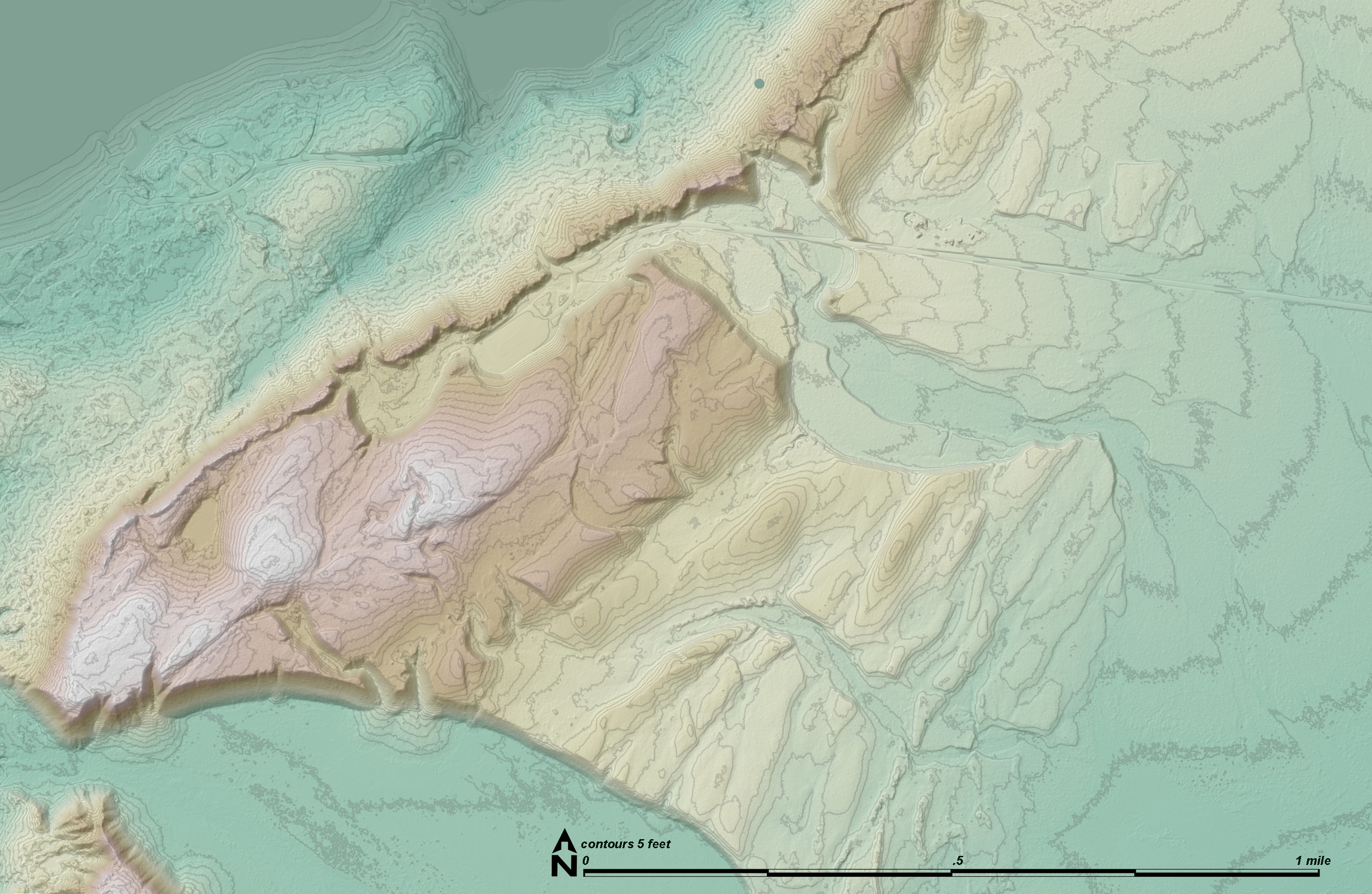
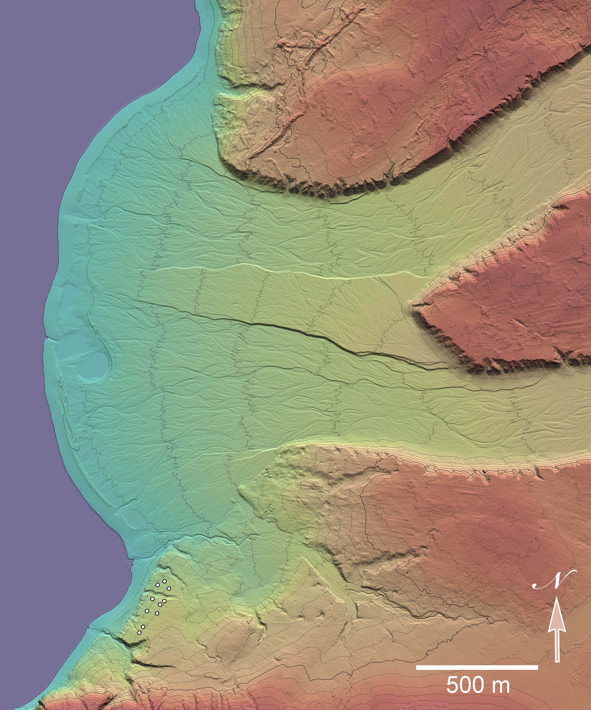
I learned about the availability of the data from Richard Carstensen who used it to make a map of the outwash channel through the peak of the 1750 terminal moraine near Park Headquarters (Figure 1). Transforming the LIDAR data into images like this requires a GIS program and some practice. The data are available for free from a USGS site and some are at a private site (a free account is required and an .edu address or other credentials make getting an account easier). I have not yet found a site with a viewer that allows you to see images made from all the new data.

Richard’s map inspired me. I set out to learn whether I could make maps like that from the new LIDAR data using a freeware GIS program (QGIS). The answer is yes, sort of. I have downloaded the “tiles” of LIDAR data near my Glacier Bay study sites in Muir Inlet and made similar maps. I have lots more to learn before my images match the pleasing quality of Richard’s map.

Figure 2. Muir Inlet, the eastern arm of upper Glacier Bay. The five thumbnails are at the youngest study sites I established between 1988 and 1990. They are labeled with the dates they were exposed from under the retreating glacier. The LIDAR maps below are of each of these sites.

Richard’s map and all of the images below are “bare earth” models of the terrain. They represent the soil or rock surface with no vegetation and reveal patterns of glacial deposition and erosion that have been hidden for decades or centuries. The colors are arbitrary and vary with elevation. Richard’s map (Figure 1) was made with the higher quality LIDAR data which is not available for any of the images below.

Figure 3. Oblique view of the 3D topographic image of the Morse Creek area. This is the fifth youngest of my 10 study sites. The 10 study plots at this site are the white dots to the right of center (ice-free by 1896). The plots are on a surface of glacial till that the glaciers slid across from right to left (north to south). Much of the till surface in this area has been washed away by meltwater pouring out of the Morse Glacier which joined the Muir Glacier here for thousands of years. As the Morse Glacier retreated (up image), its meltwater carved channels through the till. John Muir was camped across the inlet in 1890 and 1892 when glacial ice blocked the major outwash from the Morse Glacier forcing it to flow to the left around the elongate “island” of till. In about 1893 the river broke through the ice and till and flowed directly into Muir Inlet (old photos here). Today Morse Creek follows the 1893 channel. The “K” on the reddish ridge (upper center) is a possible location for Henry Fielding Reid’s Station K from which he and others observed and photographed the glaciers starting in 1892. Contour interval is 10 m.

Figure 4. Nadir (vertical) view of the terrain map of Morse Creek in Figure 3. The location of Station K is suspect because the more level bench below it (tiny white dot) is a more likely place to set up instruments for observing the glaciers. Henry Fielding Reid claimed that the station was at 620 feet (189 m) above sea level and the bench is at 540 feet (165 m). Contour interval is 10 m.

Figure 5. Topographic image of the Klotz Hills study site. White dots (lower left) are the 10 study plots (ice-free in 1910). This is a nadir (vertical) view of the image which was created from LIDAR data. The two outwash channels were carved by meltwater rivers flowing from the Casement Glacier. Today only small streams occupy these huge channels. The study plots are on a surface of glacial till that was not eroded away by the outwash. At the top of the image is an esker deposited over till while the glacier was present. It marks the course of a river flowing though or under the ice and depositing sediments in or under the ice. Contour interval is 5 m.

Figure 6. Oblique view of Goose Cove (narrow inlet left of center). White dots (center) are the 10 study plots (ice-free in 1929). The abandoned outwash channel to the right of the plots was carved by glacial meltwater from the McBride Remnant. The green triangles are approximate locations of William O. Field’s photo stations 3 (left) and 11 (top center). Some old photos from station 3 are here. Contour interval is 3 m.

Figure 7. Oblique view of the LIDAR bare earth model near the Fred study site. The 10 study plots (ice-free by 1940) are the white dots at center on a glacial till surface. The canyon-like channel was carved by glacial meltwater from the McBride Remnant. The green triangle (near plots) is the approximate location of William O. Field’s photo station 6. Some old photos from that station are here. In this image I replaced cyan with green using Photoshop because I couldn’t get it done in QGIS. Contour interval is 10 m.

Figure 8. Oblique view of the LIDAR surface model near the most recently exposed study site. There are only five study plots (white dots, ice-free in 1968) at this site but each is twice the size of plots at all other sites. The surrounding terrain is steeper than at the other Muir Inlet sites. The steep alluvial fan (center) is still modified by rain storms and seasonal snow melt from the high valley above it. The study plots are on a till surface that is still being eroded away when streamflow is high. Parts of two study plots have been lost to erosion. Contour interval is 5 m.

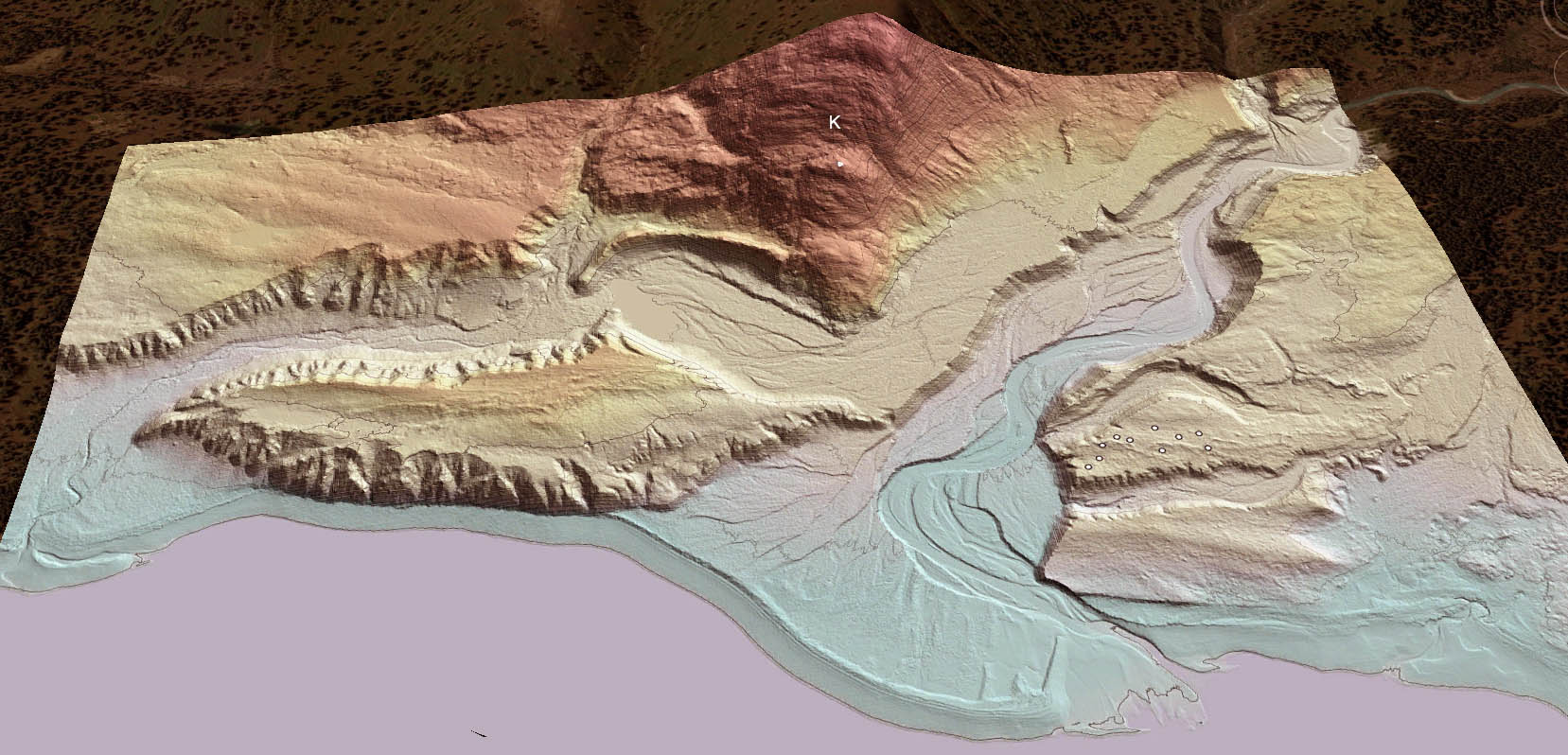
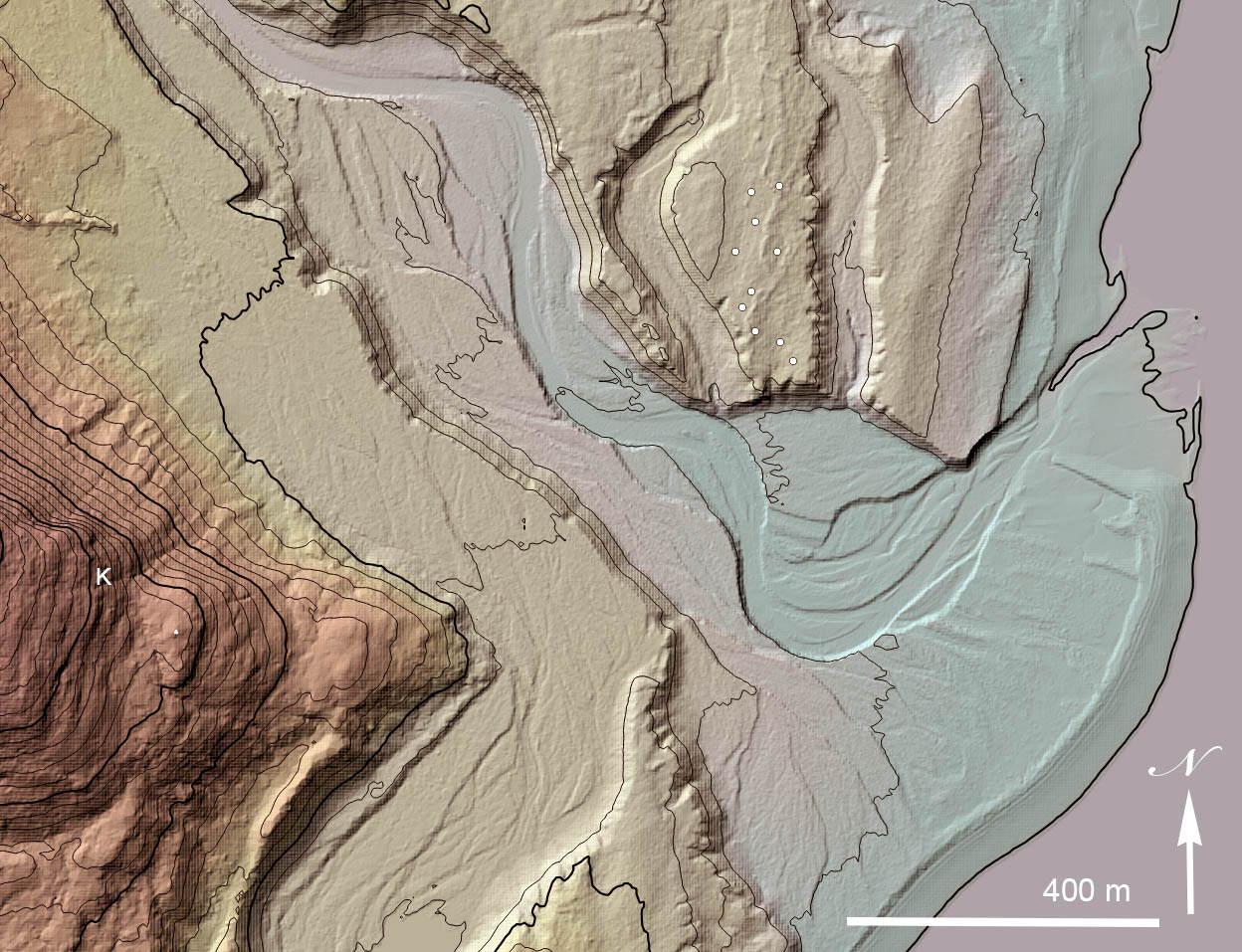
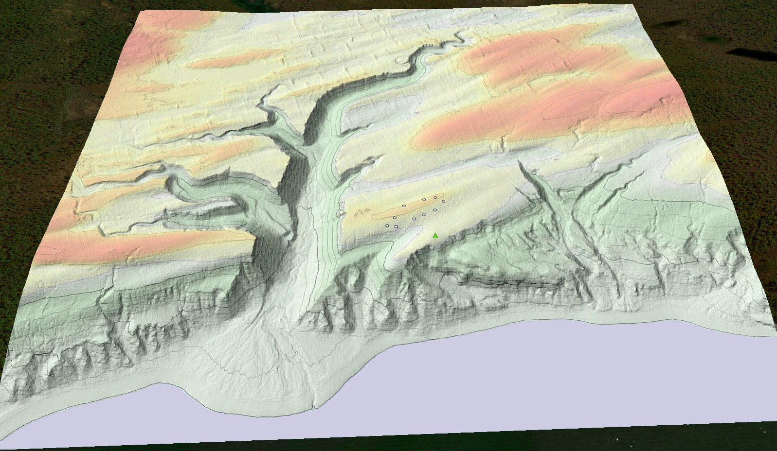
Examining the detailed LIDAR terrain surface in these images has been enlightening. There are multiple geomorphological stories at each site, one being that abandoned outwash channels and alluvial fans are everywhere. I still have to figure out how to control the display of the color gradient decorating the hillshade models in these images. I would prefer to have less of the unnatural cyan color, but have found it difficult to get rid of without resorting to Photoshop. It’s always good to have a goal.

Leave a Reply Cancel reply