The north end of Lake Dunmore is surrounded by 250 acres of flat, level land which is less than 25 feet higher than the lake. The soil is gravely sand, and lobes of sandy soil bulge into the lake at the Keewaydin and Songadeewin summer camps. I assumed these sandy lobes were deltas built into the lake as the Laurentide glacier melted away to the north, but now I’m not so sure.
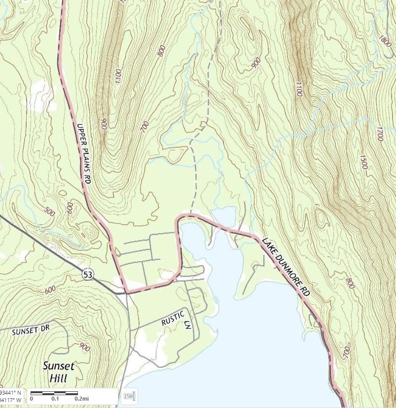
Figure 1. When I moved to this area 25 years ago this was the best map available for interpreting the history of this landscape. From this map we know that it is flat near the lakeshore north of Lake Dunmore. From the soil map we know that this flat area is gravelly sand. Learning anything else required using your legs to walk around. Camp Songadeewin is the southernmost flat area on the western side of the lake, and Camp Keewaydin is the flat peninsula on the east side. Part of USGS East Middlebury quadrangle.Continue reading “The flats and scarps of Lake Dunmore”
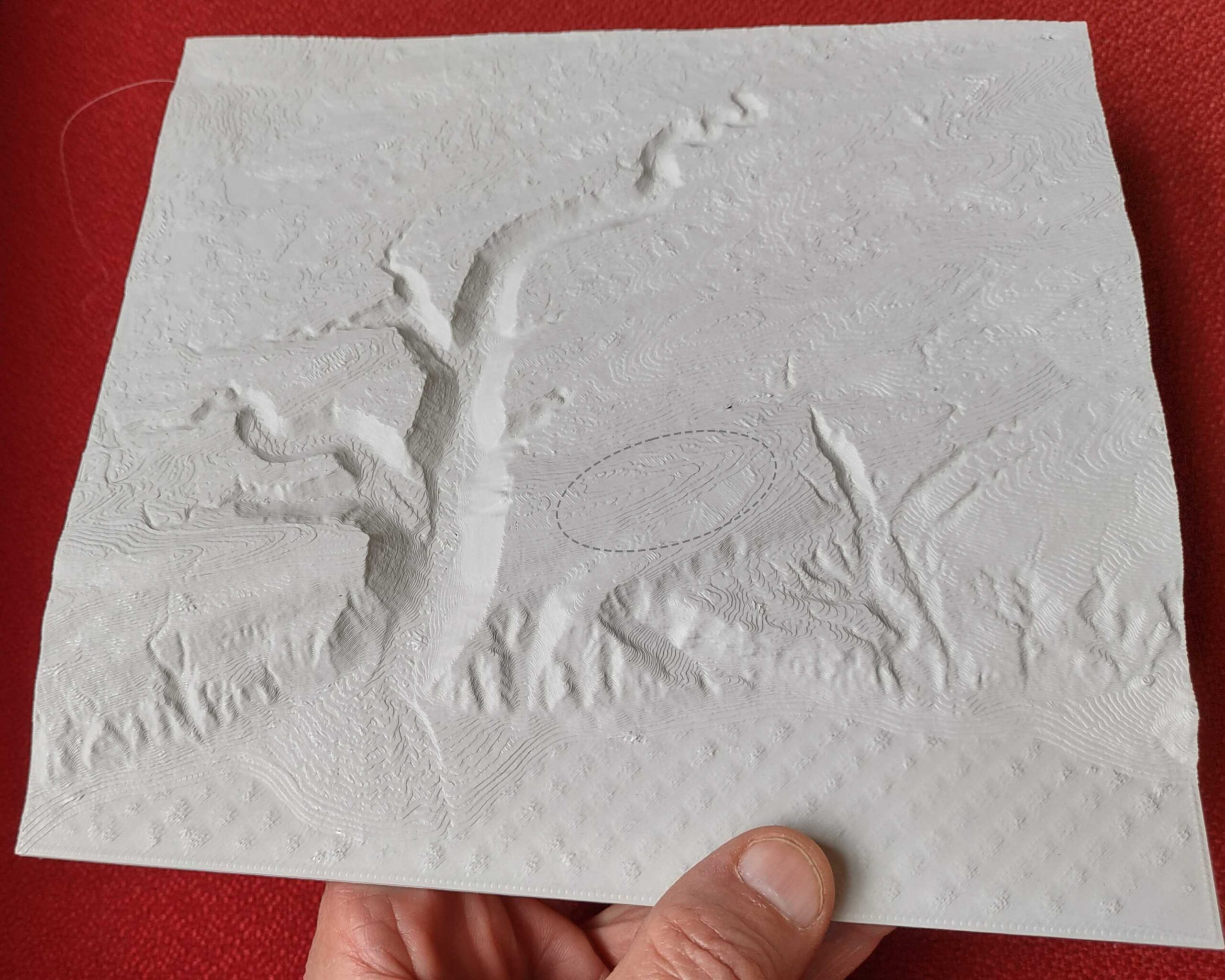
LiDAR datasets allow us to work with digital facsimiles of the earth surface and its adornments (e.g., vegetation). It’s also possible to transform the digital models back into physical form. I have been trying this with my 3D printer.
Figure 1. 3D printed relief map of the Fred study site. Ellipse is the location of 10 study plots. This is a print of the digital terrain model, or bare earth model, based on the 2019 LiDAR data from Glacier Bay. Compare Figure 7 in this previous post.The print is built by adding successive horizontal layers of plastic and the visible layers are reliable elevation contours, in this case about five foot contours.
The new LiDAR dataset for Glacier Bay includes not only the “bare earth” digital terrain model but also the point cloud which can represent vegetation and other things the airplane-borne LiDAR bounced off first before it bounced off the ground. This “first returns” cloud can show the shape of the upper vegetation canopy and even distinct understory strata. I have been trying to determine if any useful information can be quantified from the point cloud and to use QGIS to make colorful 3D images of the canopy models.
Figure 1. LiDAR first returns at Site 1 (the youngest site, emerged from the retreating glacier in 1968). Colors code for the intensity of the returned LiDAR signal. White dots are five study plots. Areas coded orange (the highest intensity) are dominated by Dryas drummondii and are present on both till and outwash. Green splotches surrounded by Dryas are cottonwood trees and willow shrubs. Blue-green clumps of vegetation are Sitka alder (circles). Gray is unvegetated outwash gravel (some of which is also blue or green). Specks (tiny squares) are noise (erroneous LiDAR returns well above the ground).Continue reading “LiDAR canopies”
In 2019 Glacier Bay National Park paid to have LIDAR mapping data collected for about a third of the park. Last summer the processed data were delivered and have now started to appear online for downloading. Most of the data are good quality (6.14 points/meter²) and the area around Park Headquarters and two areas of the outer coast (Pacific coast) are better quality (16.52 points/meter²).
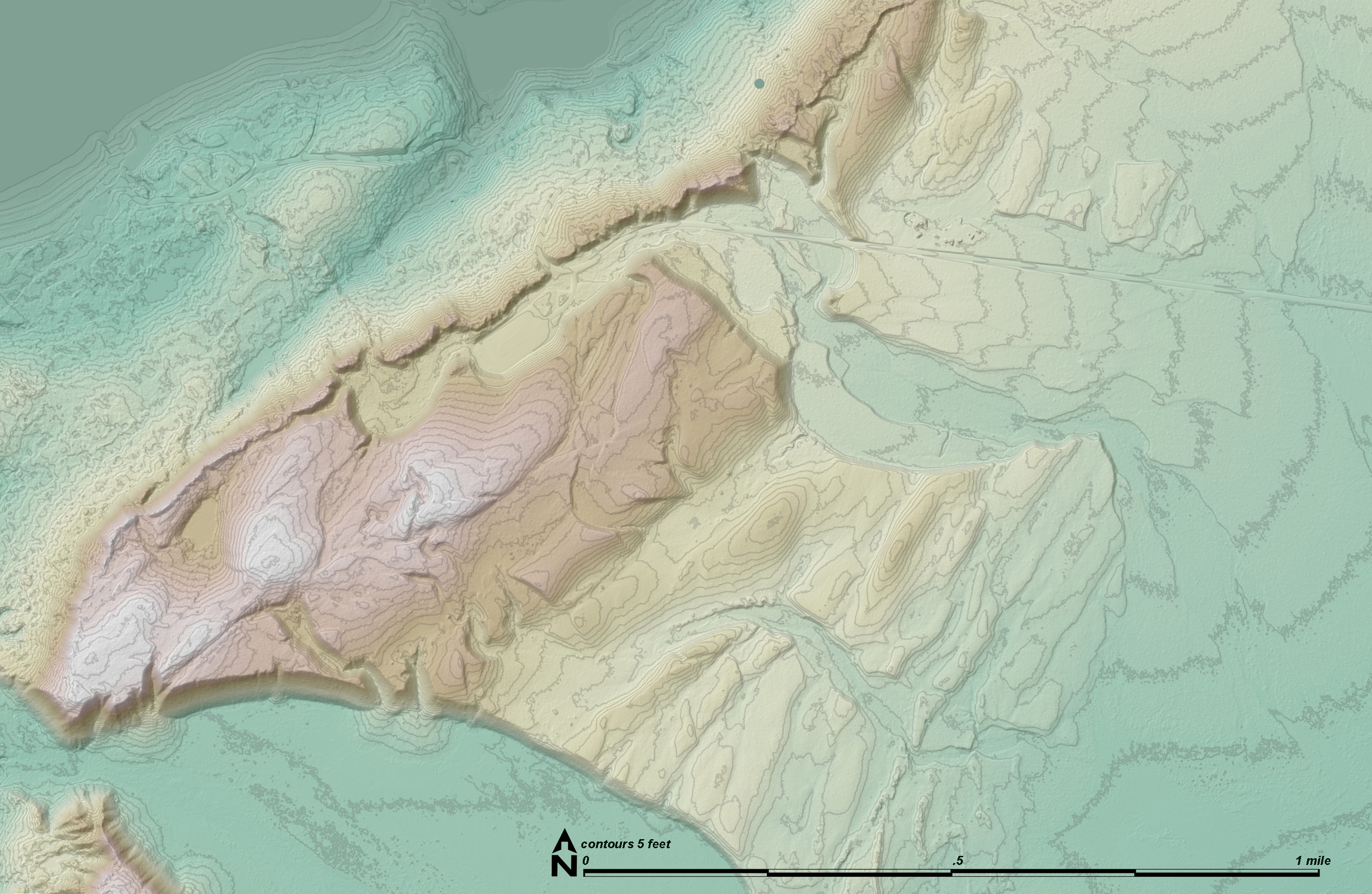
Figure 1. The 1750 terminal moraine at Bartlett Cove. Glacial ice advanced from the upper left and the front ice margin stayed at this place for long enough (a decade?) to built the ridge of sand, gravel, and boulders extending diagonally across the image. Meltwater from the glacier escaped over the moraine and eroded a channel through it and the glacial deposits in front of it (lower left). The moraine was densely forested when Europeans first studied it, so this is the first time recent scientists have been able to see the geomorphic features clearly. This map was made by Richard Carstensen using ESRI’s ArcGIS Pro software ($700/year). The downloaded LIDAR data does not look like this until much attention has been applied.Continue reading “Bare Earth surface”