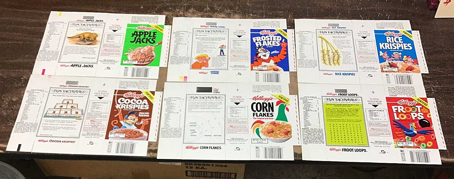
In 1992, Kellogg’s was collaborating with World Book to deliver educational content to kids on cereal boxes. In addition to its popular encyclopedia (still in print and updated every year), World Book produced Childcraft, a 15-volume set about everything interesting to kids. Childcraft produced the cereal box content.
Figure 1. Six cereal boxes (ca. 1992) from a Kellogg’s Variety Pack. Each box has a World Book Childcraft “Fun `Factivity.'” These pristine boxes were for sale on eBay.Continue reading “Fun Factivities: Daytime Darkness”
I am supposed to be curating my color slide collection so I can make thousands of digital copies that no one will ever see. I got distracted because I had to find my old slide sorting light tables and in the process also found a box with three old cameras. Two of these might have been in the family since the 1930s and the other was acquired more recently, although it is the oldest of the three.
About 10 years ago I started making digital copies of old film negatives and color slides. The scanners I had access to produced disappointing results, so I tried taking a closeup of the film with a digital camera (Figure 1). The camera was the first DSLR I owned. This made very good copies, capturing most of the information in the old film.
Figure 1. In 2013 this rig allowed me to make good copies of old 35mm film and color slides. The camera is a Nikon D40 (6 MP, model released in 2006) with an old Micro-NIKKOR 55mm 1:3.5 lens with a 12 mm extension tube. A film holder from an old enlarger holds the film or a slide.Continue reading “SliderPro 1000”
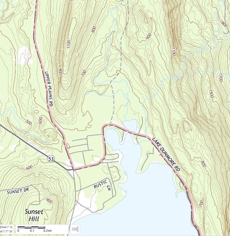
The north end of Lake Dunmore is surrounded by 250 acres of flat, level land which is less than 25 feet higher than the lake. The soil is gravely sand, and lobes of sandy soil bulge into the lake at the Keewaydin and Songadeewin summer camps. I assumed these sandy lobes were deltas built into the lake as the Laurentide glacier melted away to the north, but now I’m not so sure.
Figure 1. When I moved to this area 25 years ago this was the best map available for interpreting the history of this landscape. From this map we know that it is flat around this part of Lake Dunmore. From the soil map we know that this flat area is gravelly sand. Learning anything else required walking around. Camp Songadeewin is the southernmost flat area on the western side of the lake, and Camp Keewaydin is the flat peninsula on the east side. Part of USGS East Middlebury quadrangle.Continue reading “The flats and scarps of Lake Dunmore”
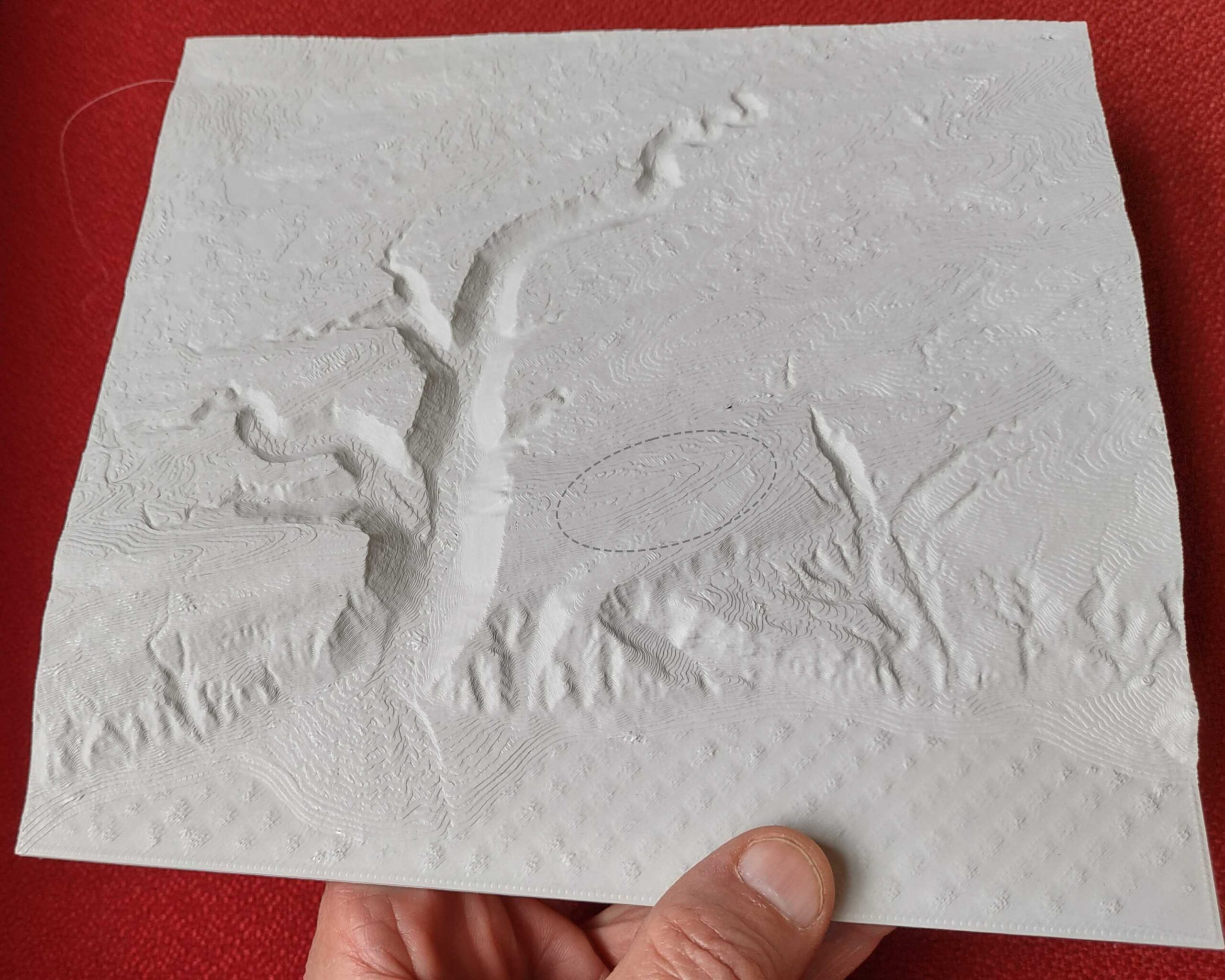
LiDAR datasets allow us to work with digital facsimiles of the earth surface and its adornments (e.g., vegetation). It’s also possible to transform the digital models back into physical form. I have been trying this with my 3D printer.
Figure 1. 3D printed relief map of the Fred study site. Ellipse is the location of 10 study plots. This is a print of the digital terrain model, or bare earth model, based on the 2019 LiDAR data from Glacier Bay. Compare Figure 7 in this previous post.The print is built by adding successive horizontal layers of plastic and the visible layers are reliable elevation contours, in this case about five foot contours.
The new LiDAR dataset for Glacier Bay includes not only the “bare earth” digital terrain model but also the point cloud which can represent vegetation and other things the airplane-borne LiDAR bounced off first before it bounced off the ground. This “first returns” cloud can show the shape of the upper vegetation canopy and even distinct understory strata. I have been trying to determine if any useful information can be quantified from the point cloud and to use QGIS to make colorful 3D images of the canopy models.
Figure 1. LiDAR first returns at Site 1 (the youngest site, emerged from the retreating glacier in 1968). Colors code for the intensity of the returned LiDAR signal. White dots are five study plots. Areas coded orange (the highest intensity) are dominated by Dryas drummondii and are present on both till and outwash. Green splotches surrounded by Dryas are cottonwood trees and willow shrubs. Blue-green clumps of vegetation are Sitka alder (circles). Gray is unvegetated outwash gravel (some of which is also blue or green). Specks (tiny squares) are noise (erroneous LiDAR returns well above the ground).Continue reading “LiDAR canopies”
In 2019 Glacier Bay National Park paid to have LIDAR mapping data collected for about a third of the park. Last summer the processed data were delivered and have now started to appear online for downloading. Most of the data are good quality (6.14 points/meter²) and the area around Park Headquarters and two areas of the outer coast (Pacific coast) are better quality (16.52 points/meter²).
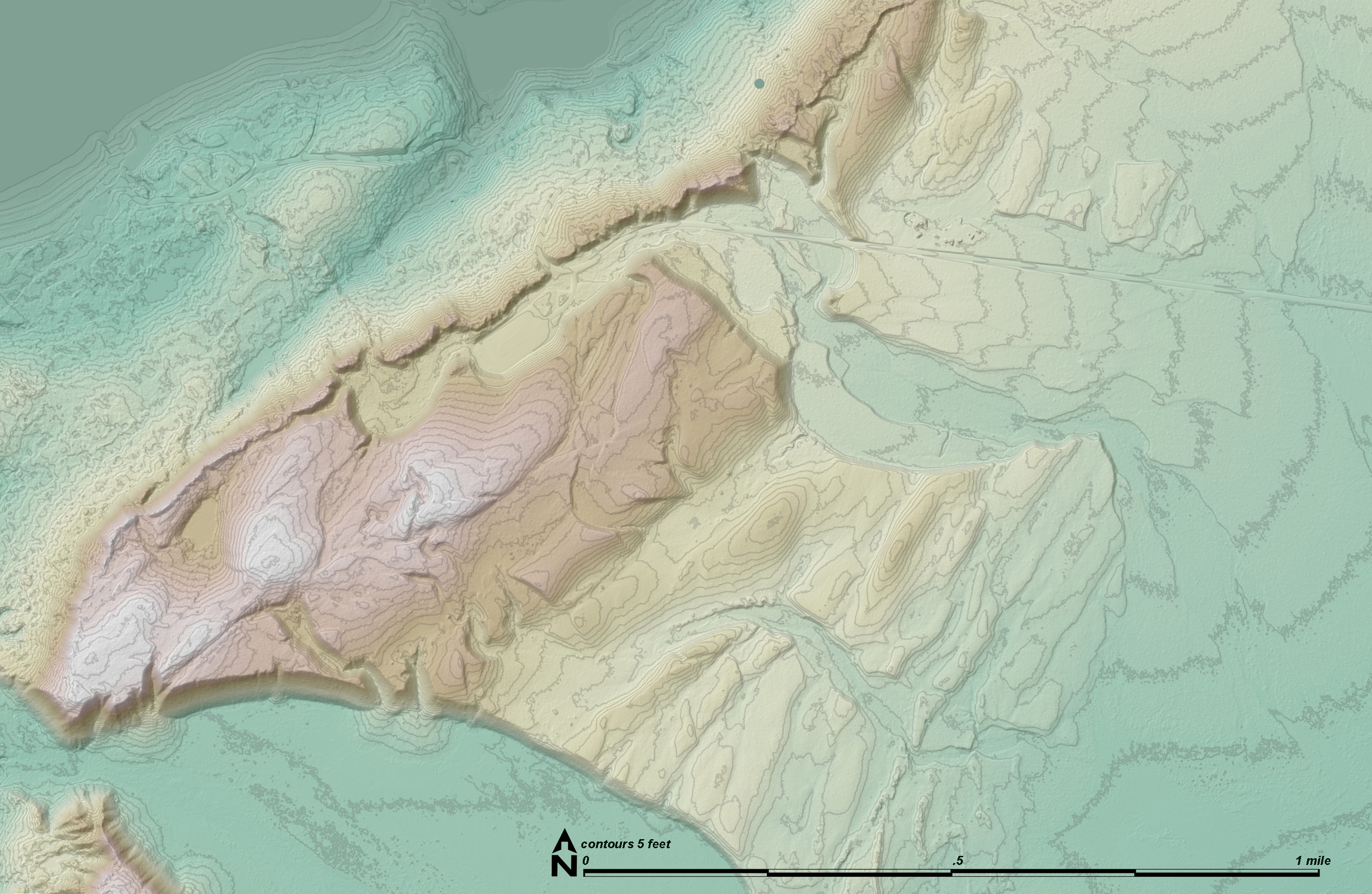
Figure 1. The 1750 terminal moraine at Bartlett Cove. Glacial ice advanced from the upper left and the front ice margin stayed at this place for long enough (a decade?) to built the ridge of sand, gravel, and boulders extending diagonally across the image. Meltwater from the glacier escaped over the moraine and eroded a channel through it and the glacial deposits in front of it (lower left). The moraine was densely forested when Europeans first studied it, so this is the first time recent scientists have been able to see the geomorphic features clearly. This map was made by Richard Carstensen using ESRI’s ArcGIS Pro software ($700/year). The downloaded LIDAR data does not look like this until much attention has been applied.Continue reading “Bare Earth surface”
The Fred and Goose Cove study sites at Glacier Bay are only 4.2 km (2.7 miles) apart and the glacier exposed Goose Cove only about a decade earlier than Fred. The vegetation development at Goose Cove during the two decades after I established the plots (ca. 1990-2010) should be comparable to the most recent two decades of development at Fred (ca. 2000-2020). Precise comparisons require that I know how old the two sites are.
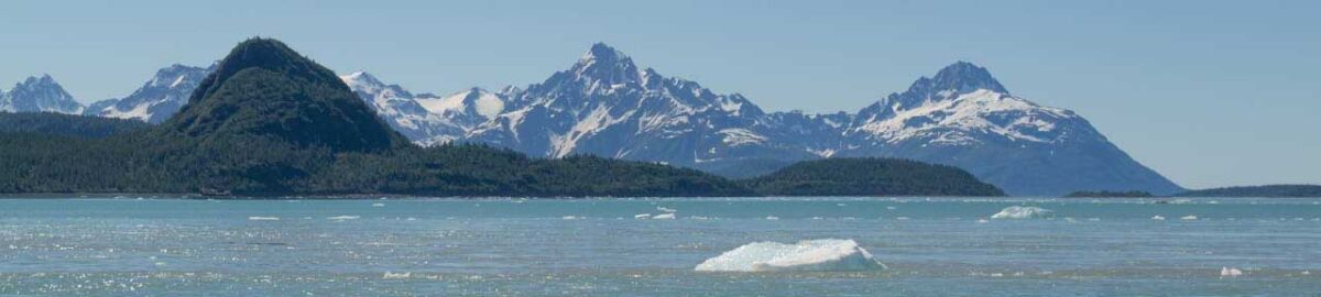
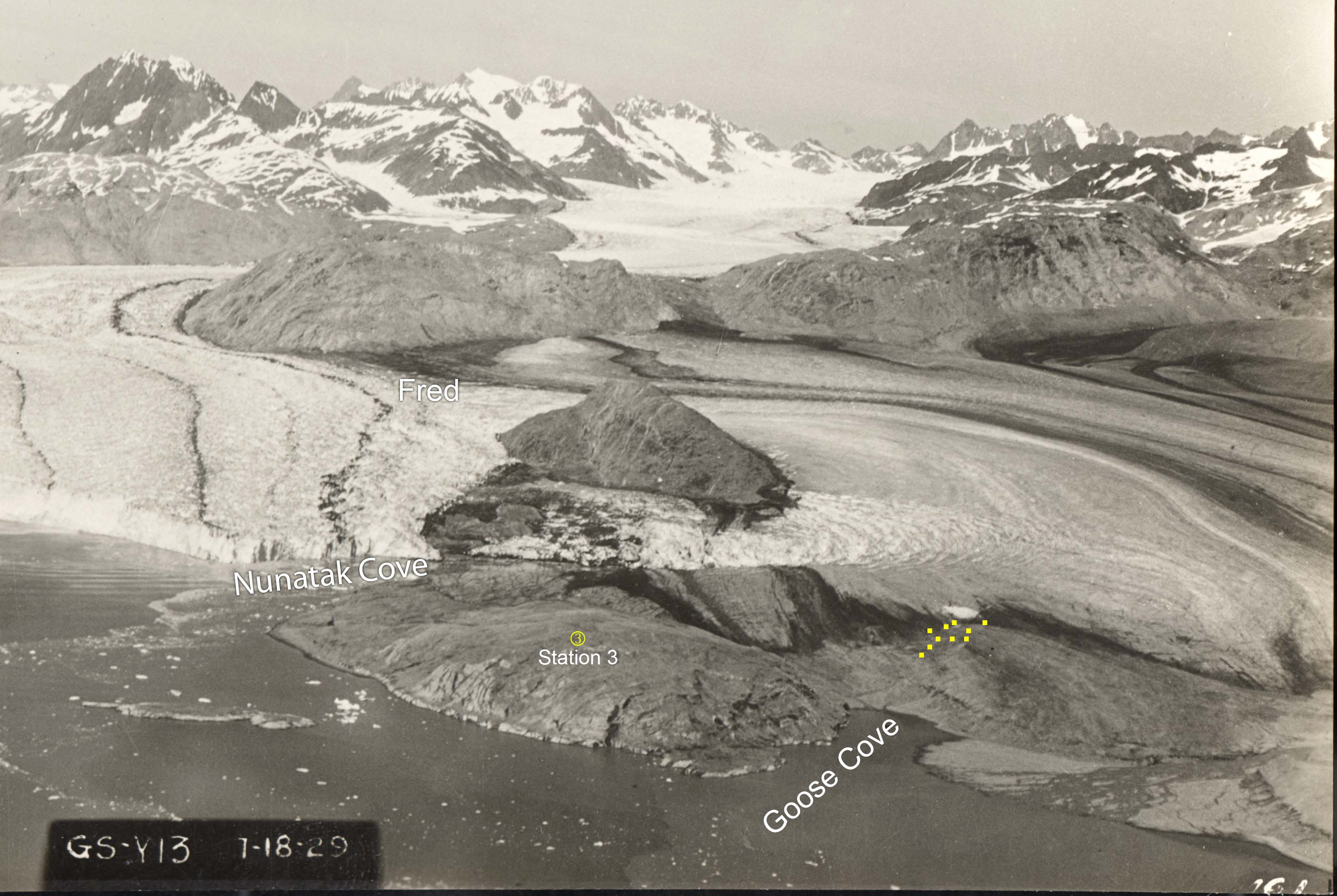
Figure 1. Oblique aerial photo of the Muir Glacier (left) and the stagnating mass of the McBride Glacier (right) in July, 1929. Goose Cove is free of ice and the study plots established in 1988 (yellow squares) are mostly free of ice. Station 3 is one of William O. Field’s photo stations. NSIDC Digital File ID: muir1929071801.Continue reading “Have photo – will date”
The second youngest of my 10 study sites at Glacier Bay is called Fred because there is a USGS benchmark there named Fred. Fred is dominated by alder. When the plots were established in 1988, there were no spruce and the average diameter of the cottonwood trees was 7 cm (2.8 inches). There were about five of these little cottonwood trees in each plot and 280 alder stems. There are 10 plots and we measured the diameter of all 2800+ stems.
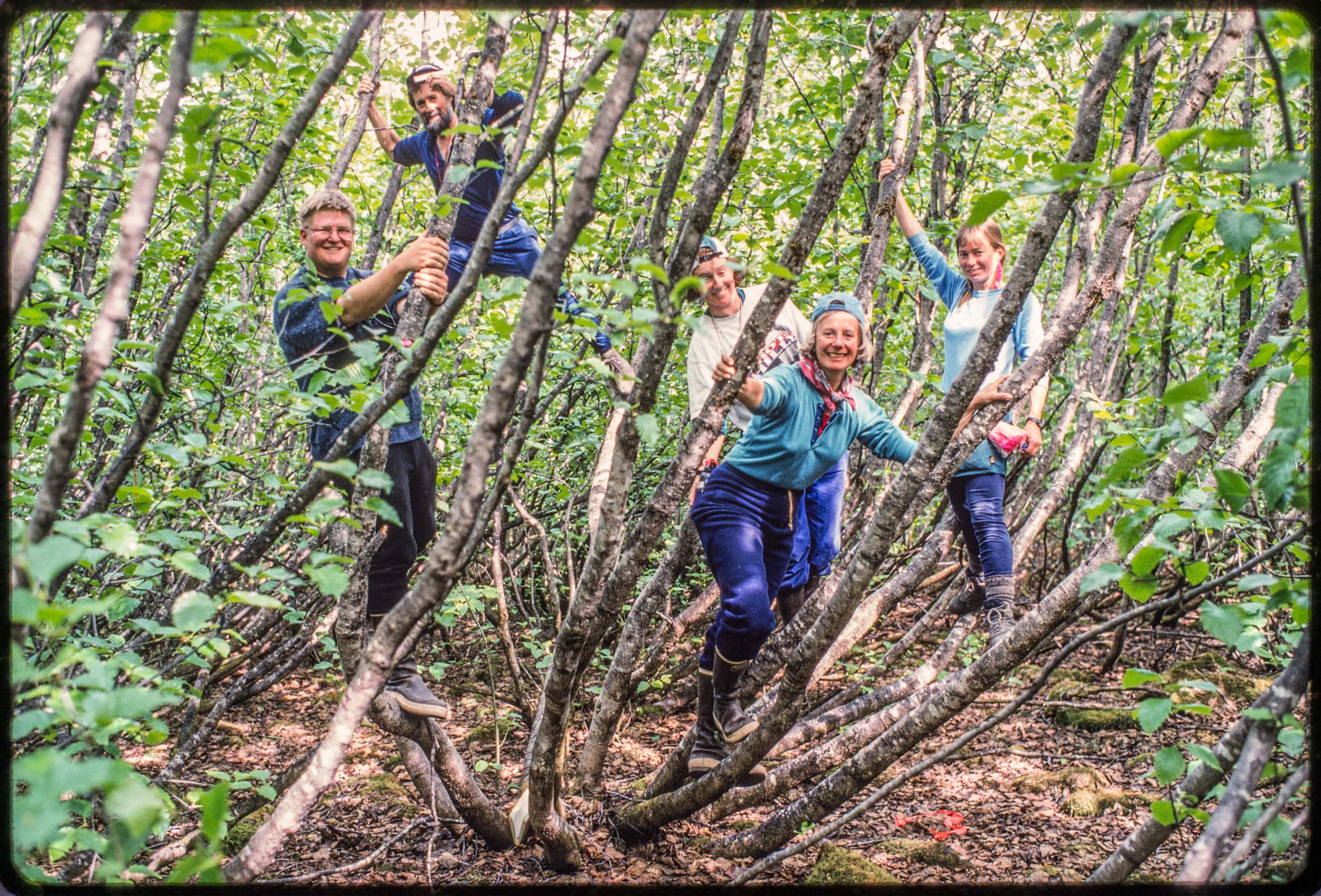
Figure 1. The 1995 field crew in Mother Alder in plot 4 at Fred. This alder was substantially larger and older than any other in the plots and probably begat many of its neighbors. Left to right: Jim Speer, Gary Bolton, Andi Lloyd, Ginger Burley, Elise Pendall. Kodachrome, May 24, 1995.
The primary source I used to date Fred’s emergence from under the glacier was an aerial photo taken in 1948. The McBride remnant, a large extent of shrinking, stagnant ice, was 550 m away from the plots and I guessed that four years earlier the ice had probably covered the plots. I was probably off by a few years.
Three decades ago I started monitoring vegetation change in Glacier Bay National Park where glaciers have been retreating and exposing new land to colonization by plants. Each of the 10 sites I study was exposed at a different date over the last 250 years and it’s important to know that date for each site. It seems even more important now that I have so much data from the sites.
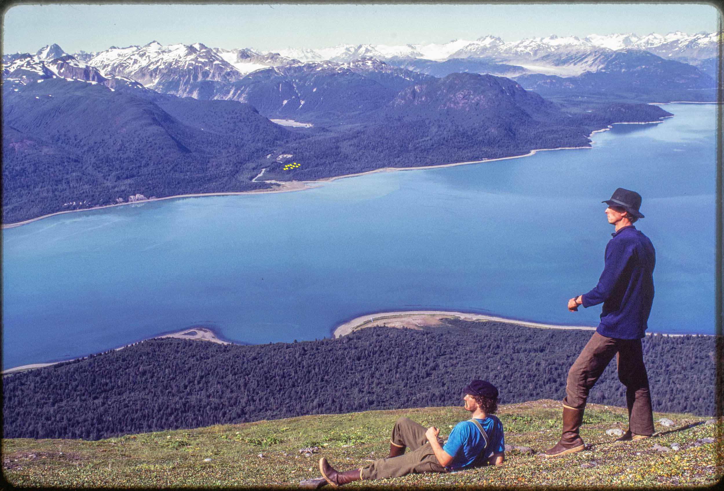
Figure 1. The view of Muir Inlet from 2000 feet above Muir Point on the shoulder of Mount Wright. Across the inlet are 10 tiny yellow squares where the Morse Creek study site is. We established those study plots near Morse Creek in 1988 without knowing exactly when the glacial ice had melted away there. Foreground: Left; H. Lentfer, Right; author. Kodachrome slide, August 1988. Continue reading “Dating retreat”
More than a year ago I took a hike along the Green Mountain Escarpment (Vermont) in search of an old mine. I had read in an old report that Indiana bats hibernated in a mine in the area, and that was enough of an excuse to go exploring. I watched a bear and two cubs for 15 minutes but never found a mine. It was a pleasant hike along old logging roads through private property. No one lived on the several properties I traversed, none of which was posted.
Figure 1. This six acre wetland is at the base of the steep, rocky slopes I was exploring for a mine. Although I found nothing on the slopes resembling a bat hibernaculum, this wetland looked like excellent foraging habitat for bats. Plants in bloom include Canada goldenrod, jewelweed, boneset, joe pye weed, and New England aster. September 11, 2020.Continue reading “Indiana Bats and the Grotto of Doom”
After 12 nights of recording bat calls near an Indiana bat maternity roosting colony, we deployed the AudioMoths for a week at the vernal pool where we recorded bat calls in August. Instead of putting two AudioMoths at the vernal pool, we put one by the pool and two in the forest surrounding the pool. One of the forest AudioMoths recorded nothing (a battery was inserted backwards), so we got data from only one non-pool AudioMoth.
Figure 1. Vernal pool MLS619 (Bridport, VT) on September 23, 2021 at the end of a week of recording bat calls. There was no standing water in the pool but the liquid mud was 6 inches deep. This might be as low as the water level gets in the pool this year (it was dry and firm last October). There were a few inches of water in the pool at the beginning of the AudioMoth recording on September 16.Continue reading “More noise, fewer bats”