The new LiDAR dataset for Glacier Bay includes not only the “bare earth” digital terrain model but also the point cloud which can represent vegetation and other things the airplane-borne LiDAR bounced off first before it bounced off the ground. This “first returns” cloud can show the shape of the upper vegetation canopy and even distinct understory strata. I have been trying to determine if any useful information can be quantified from the point cloud and to use QGIS to make colorful 3D images of the canopy models.
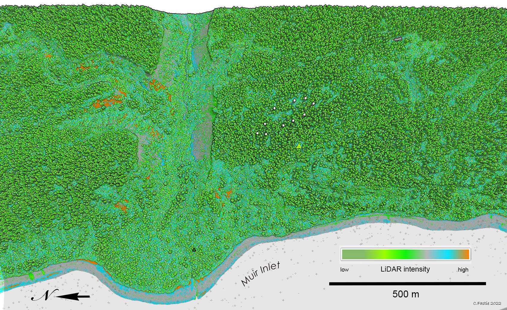
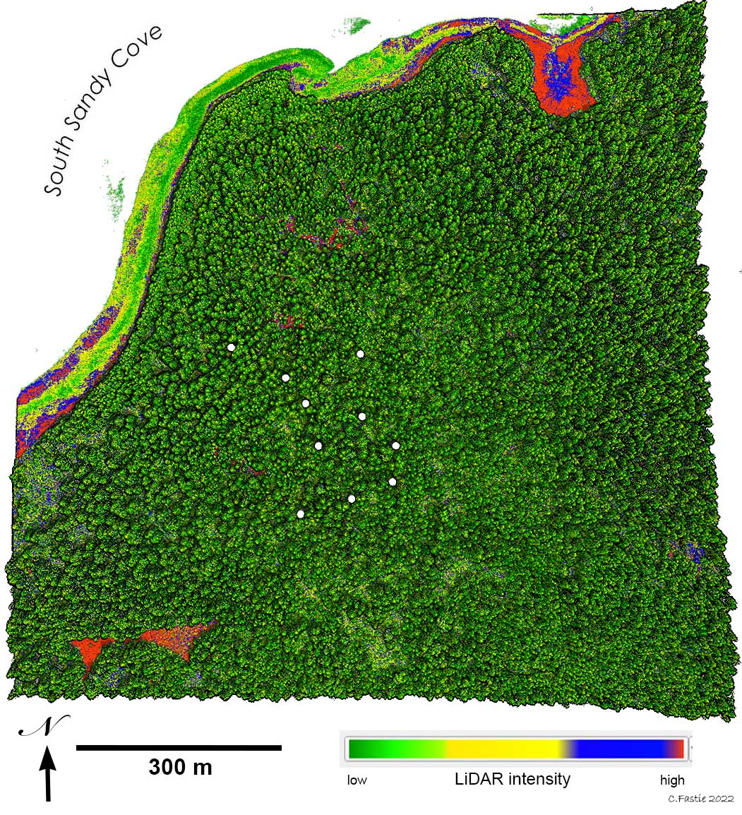
Figure 1. LiDAR first returns at Site 1 (the youngest site, emerged from the retreating glacier in 1968). Colors code for the intensity of the returned LiDAR signal. White dots are five study plots. Areas coded orange (the highest intensity) are dominated by Dryas drummondii and are present on both till and outwash. Green splotches surrounded by Dryas are cottonwood trees and willow shrubs. Blue-green clumps of vegetation are Sitka alder (circles). Gray is unvegetated outwash gravel (some of which is also blue or green). Specks (tiny squares) are noise (erroneous LiDAR returns well above the ground).Figure 2. Ten study sites along the east side of Glacier Bay. Images of the canopy height model from LiDAR first return data for eight of the 10 sites are included here. Years are when each site emerged from under the retreating glacier. Colors of symbols code for successional pathway (see Figures 3 and 5 below).
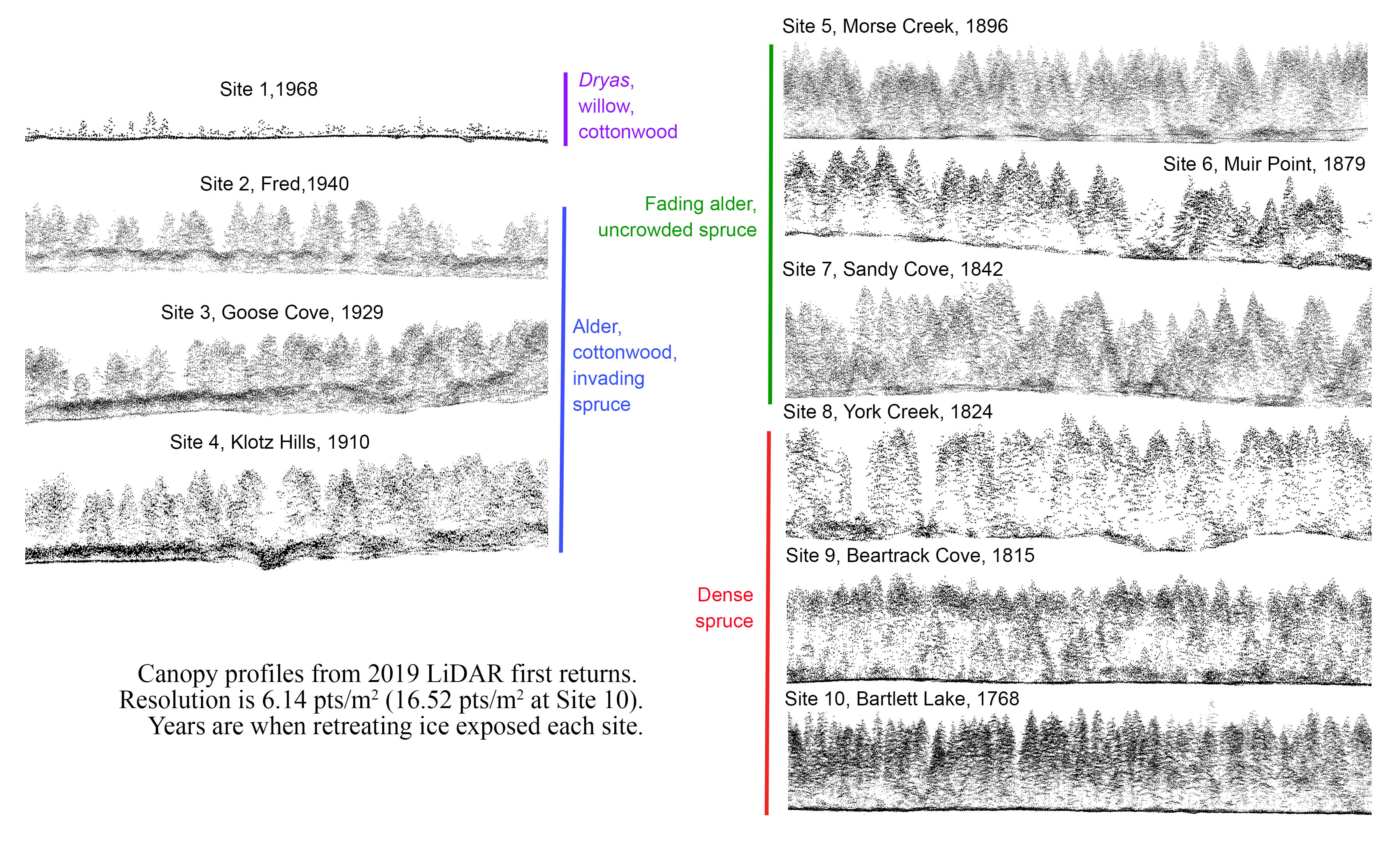
It’s also possible to look at vertical profiles through the point cloud. These often show individual trees especially in the upper canopy. The shape of the tree canopy is revealed, but it is more difficult to distinguish cottonwood from spruce than I would have expected.
Figure 3. Sample canopy profiles from 10 study sites. These images were made with FugroViewer which displays LiDAR point clouds and vertical profiles of them. Site 1: the taller plants are black cottonwood trees and others are willow shrubs. Sites 2-4: The tree canopy is mostly cottonwood, and below it is a conspicuous alder canopy. Sites 5-7: The tree canopy is almost all Sitka spruce, with alder shrub canopies evident especially under canopy gaps. Sites 8-10: Canopies are primarily spruce and much denser than at younger sites. The tallest trees are at Sandy Cove and York Creek (Sites 7 and 8).
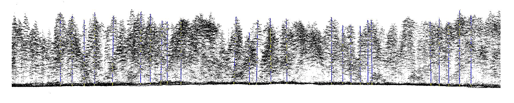
The canopy profiles maintain the precise height measurements of the LiDAR data so it is possible to measure tree height. I tried this in multiple profiles at each of my 10 study sites. I systematically selected sampling points along the transects and measured the height of five trees closest to each point.
Figure 4. Canopy profile from the Bartlett Lake study site. Blue lines are canopy height measurements made in FugroViewer. Five sampling points were equally spaced along the transect and the closest five trees with obvious crowns were measured. The width of the belt transect was generally 20-30 m.
I measured tree height along three transects at Sites 5-10 where the trees are mostly Sitka spruce and along two transects at Sites 1-4 where the trees are mostly cottonwood. I measured a total of 650 tree heights.
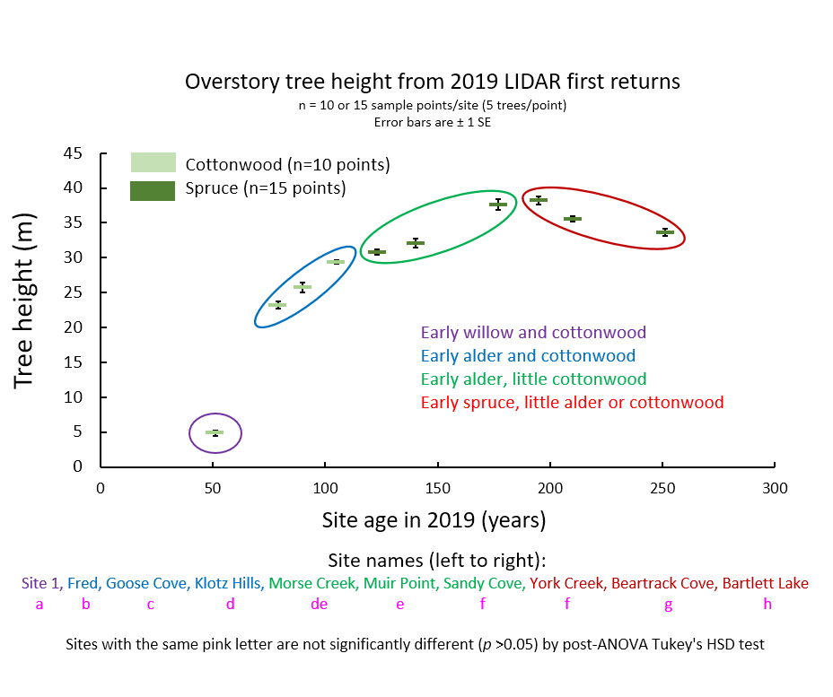
Figure 5. Mean tree height at 10 study sites from measurements of LiDAR canopy profiles. Sites are grouped (ellipses) by successional pathway. Differences among sites were determined using R.
The tallest spruce are at Sandy Cove and York Creek (Sites 7 and 8). There are more trees at York Creek and they have bigger basal diameters, so the basal area (cross-sectional tree trunk area per unit area of forest) is 50% greater at York Creek compared to Sandy Cove. The two older sites have shorter spruce trees probably because the trees are much more densely packed, the soil is less well-drained, and alders never fixed much nitrogen there.
The tree height comparisons are useful because they follow a pattern with site age that is followed by other parameters — something we measure (tree height, biomass, carbon pools, nitrogen) increases along a sequence of progressively older sites until the oldest sites near the mouth of the bay where we measure less of it. This might be the actual time course at a site for some other parameters, but it is less likely that tree height will decrease with time. Average tree height can decline if the tallest trees die, but there is no indication that this has happened at these sites. Spruce bark beetles probably killed some trees at the older sites, but those trees were more likely the slower growing trees that had captured less of a place in the sunny overstory, not the tallest trees. So it makes sense that the decline with tree height along the chronosequence is not something that happened, or will happen, at any single site in its first three centuries. It is an incorrect inference from a flawed chronosequence.
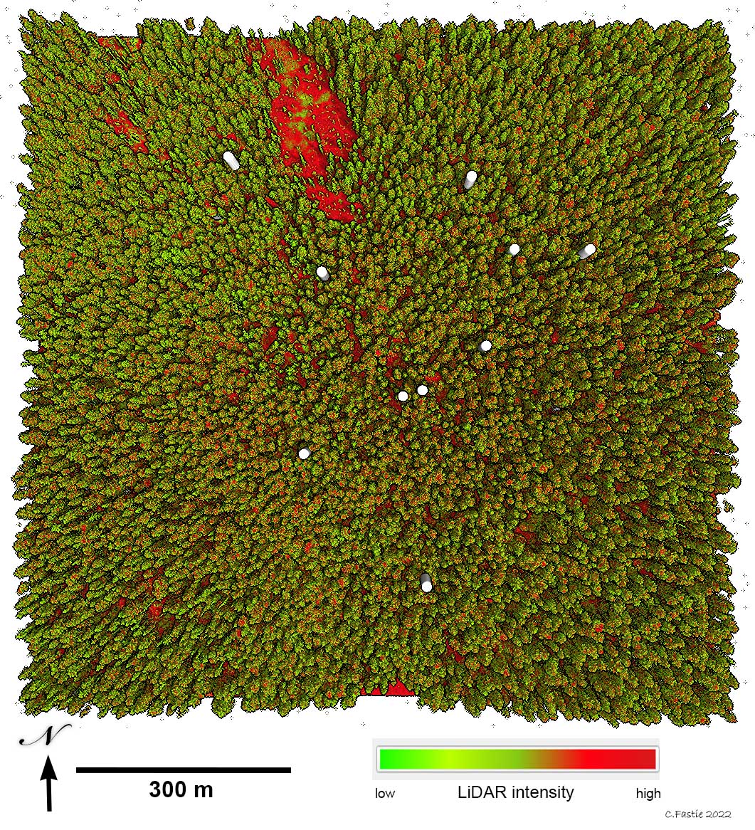
Figure 6. LiDAR canopy height model at Site 2 (Fred, exposed in 1941). Colors code for the intensity of the LiDAR signals. White dots are 10 study plots. There are no canopy spruce in the study plots at this site so almost all of the trees are cottonwood. The bluer color among the trees is the shrub canopy dominated by alder. Orange is mostly Dryas drummondii which is slowly being eliminated by encroaching alders. The green triangle (near study plots) is the approximate location of William O. Field’s photo station 6. The black triangle (on outwash fan) is the approximate location of a USGS very accurate bench mark (VABM) named “Fred.”
Coloring the canopy models as a function of the intensity of the LiDAR returns allows some of the important plant species to be distinguished. Dryas drummondii returns a very strong signal and is faithfully distinguished at some sites (Figures 1 and 6). However, supratidal meadows also have high intensity LiDAR returns (Figures 7 and 8) and do not include Dryas. Alder tends to return a stronger signal than willow or cottonwood and can sometimes be distinguished from them.
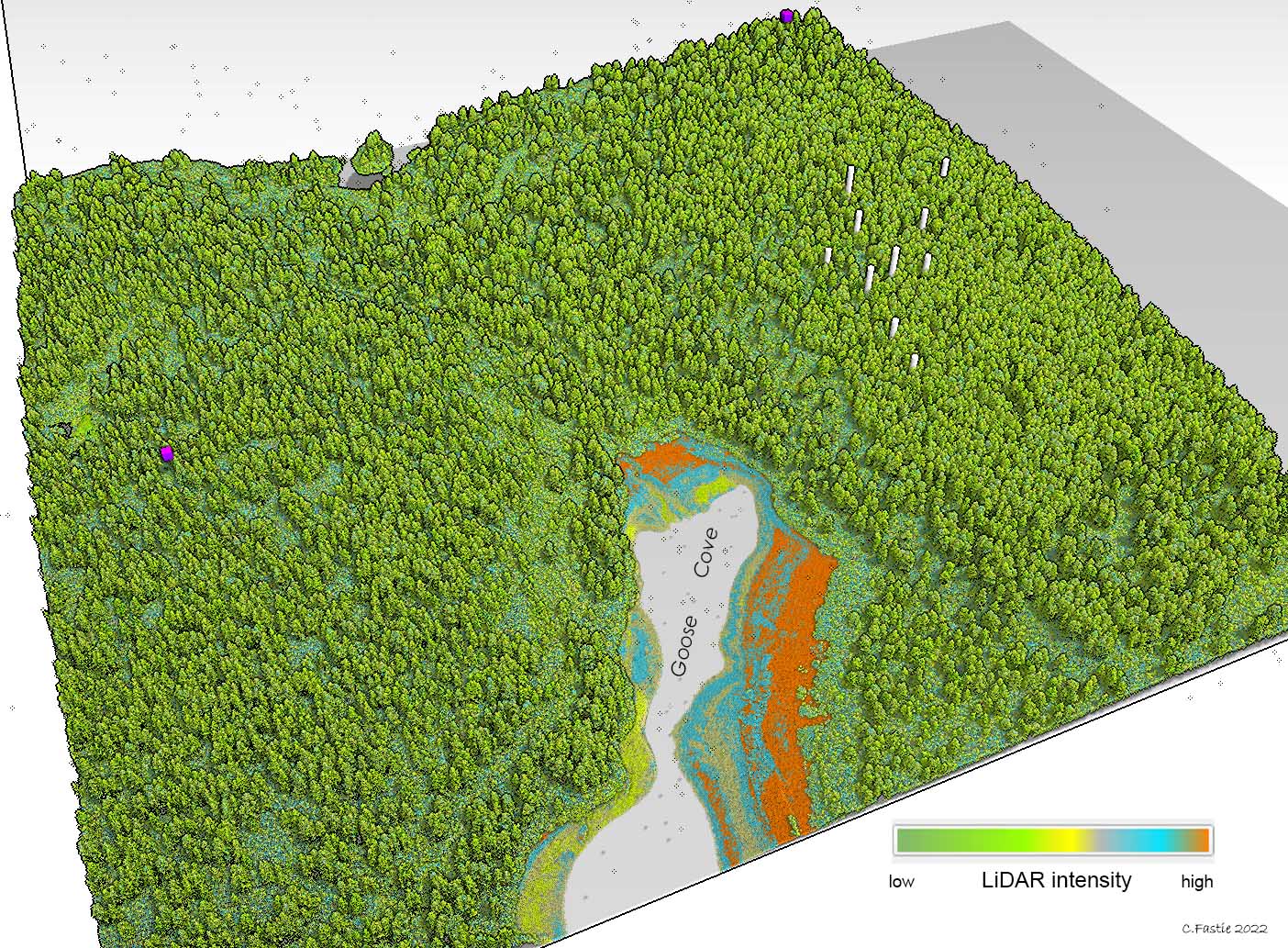
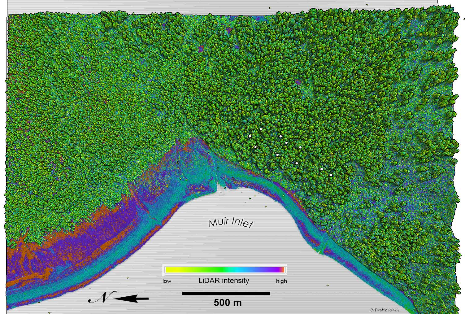
Figure 7. LiDAR canopy height model at Site 3 (Goose Cove, exposed in 1929). Colors code for the intensity of the LiDAR signals. This is an oblique view (the only image here that is not a nadir view). White columns are 10 study plots. Most of the trees are cottonwood. The lower bluer canopy is alder. Supratidal meadows produce the strongest LiDAR reflection (orange). Purple cubes are William O. Field’s photo stations 3 (left) and 11 (top).Figure 8. LiDAR canopy height model at Site 4 (Klotz Hills, exposed in 1910). Colors code for the intensity of the LiDAR signals. White dots are 10 study plots. More than half of the canopy trees are cottonwood and the rest are spruce. The bluer, finer-textured canopy is alder. Supratidal meadows have the strongest LiDAR signals (blue and orange). The left half of the image is an outwash fan that is younger than the area of the study plots and has smaller, shorter cottonwood and spruce trees.
Sites pictured above (Sites 1-4) do not yet have continuous tree canopies. Canopy gaps show remnants of the shrub thicket that is slowly deteriorating as trees overshadow it. Sites pictured below (Sites 5,7,8,10) have almost continuous canopies of Sitka spruce (there are a few cottonwoods at Site 5 and a few hemlocks at Site 10). The four figures below illustrate the variability in spruce density and canopy homogeneity. Site 10 (Figure 12) has more spruce per unit area and the trees appear to be distributed more evenly that at younger sites.
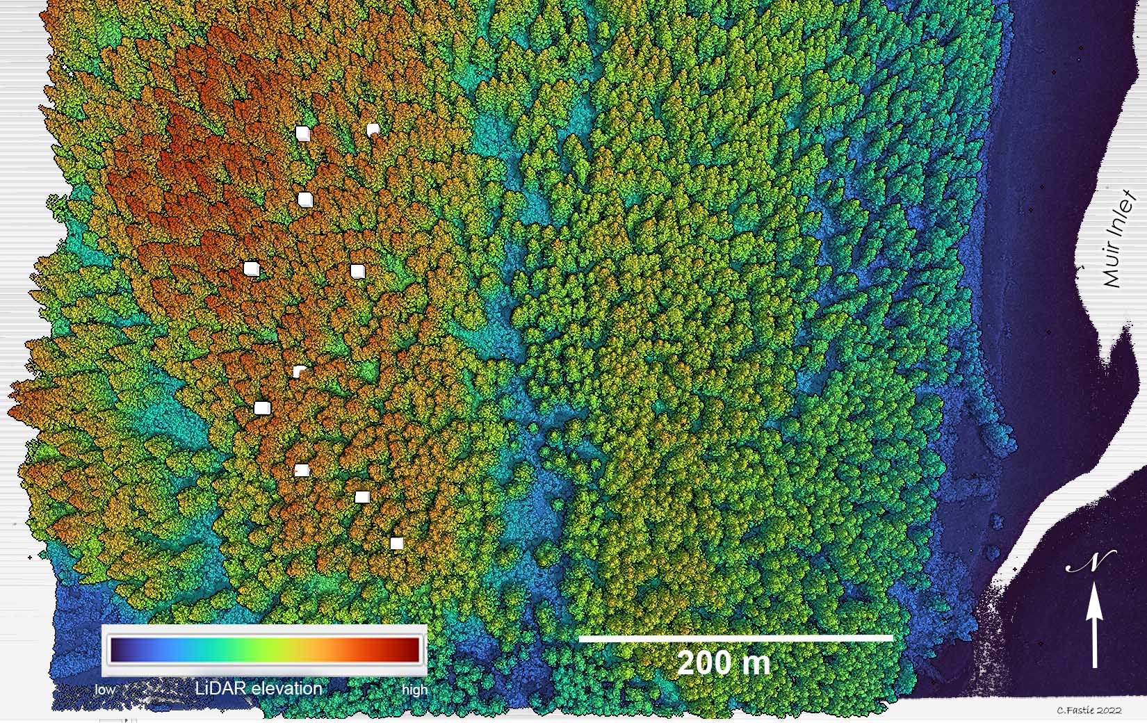
Figure 9. Color-coded image of a canopy height model at the Morse Creek study site (Site 5, exposed in 1896). Most of the trees are Sitka spruce. White squares are 10 study plots. The blue area bisecting the image vertically is the Valley of the Stumps (has many exposed remnants of standing trees buried by outwash as the glacier advanced). Colors code for elevation above sea level (not canopy height above the ground). Only one other image below is color-coded for elevation (Figure 11).Figure 10. LiDAR canopy height model at Site 7 (Sandy Cove, exposed in 1842). Colors code for the intensity of the LiDAR signals. White dots are 10 study plots. The orange and blue area (upper right) includes a large Carex lyngbyei meadow.Figure 11. LiDAR canopy height model at Site 8 (York Creek, exposed in 1824). Colors code for elevation above sea level (not canopy height). White dots are 10 study plots. Almost all trees are Sitka spruce which are denser than at any younger site but not as dense as at Sites 9 and 10. The York Creek study plots have the greatest tree basal area and biomass of the 10 study sites (and probably the tallest trees, Figure 5).Figure 12. LiDAR canopy height model at Site 10 (Bartlett Lake, exposed in 1796). Colors code for the intensity of the LiDAR signals. White columns are 10 study plots. Spruce trees are denser here than at sites in the figures above (Site 9, Beartrack Cove, has denser spruce). The red area (top) is a shallow pond and wetland that appears to have spread in the last 30 years probably through the process of palludification.
Quantifying tree heights from the LiDAR data seems to have promise. I did not make field measurements of tree height at my study plots very often, so even the simple tree height exercise described here provides useful information about differences among sites. The technique I used does not scale well, but skilled GIS practitioners can produce a continuous map of canopy height values. This can then be used to produce mean canopy heights at any scale for any subset of the landscape.
There are other parameters that could be measured or modeled, e.g., canopy texture, canopy tree density, or tree biomass. I don’t see a pressing need to pursue these metrics at my Glacier Bay sites.
The real power of this type of data might be realized in a decade or two when the data collection is repeated either with LiDAR or some new technology. Then the fate of individual trees could be followed and long-term changes in tree height, canopy width, tree density, or biomass can be documented. The timing might be good if I want to continue monitoring the study sites because by that time they won’t be letting me out of the home.
3 thoughts on “LiDAR canopies”
The specifications I found for the Glacier Bay LiDAR are 6.14 points/meter² for most of it. The area around Park Headquarters and two areas of the outer coast are better quality (16.52 points/meter²). Do you know why those areas on the outer coast got better quality LiDAR?


The specifications I found for the Glacier Bay LiDAR are 6.14 points/meter² for most of it. The area around Park Headquarters and two areas of the outer coast are better quality (16.52 points/meter²). Do you know why those areas on the outer coast got better quality LiDAR?
Where on the outer coast?
How dense are LiDAR returns? Say, from bare ground. Some metric like number of points per square meter (or square centimeter).