LiDAR datasets allow us to work with digital facsimiles of the earth surface and its adornments (e.g., vegetation). It’s also possible to transform the digital models back into physical form. I have been trying this with my 3D printer.
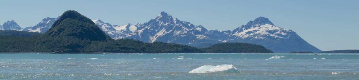
I started printing 3D relief maps a few years ago with coarser data. There are several websites where you can download printer-ready (.stl) files of user-selected map areas in most of the US. This summer I found some coarse data for Glacier Bay and printed a five inch (13.5 cm) wide model of the bay. Acrylic artist’s paints work well to decorate the printed maps.

Last fall I learned that opentopography.org was making high resolution LiDAR data available for many areas. Glacier Bay was not yet included, but the potential for printing detailed, small-scale relief maps encouraged me to buy a larger 3D printer (20 cm x 25 cm [8 in x 10 in] build area). Even with old, coarse data a bigger printer can produce impressive results.
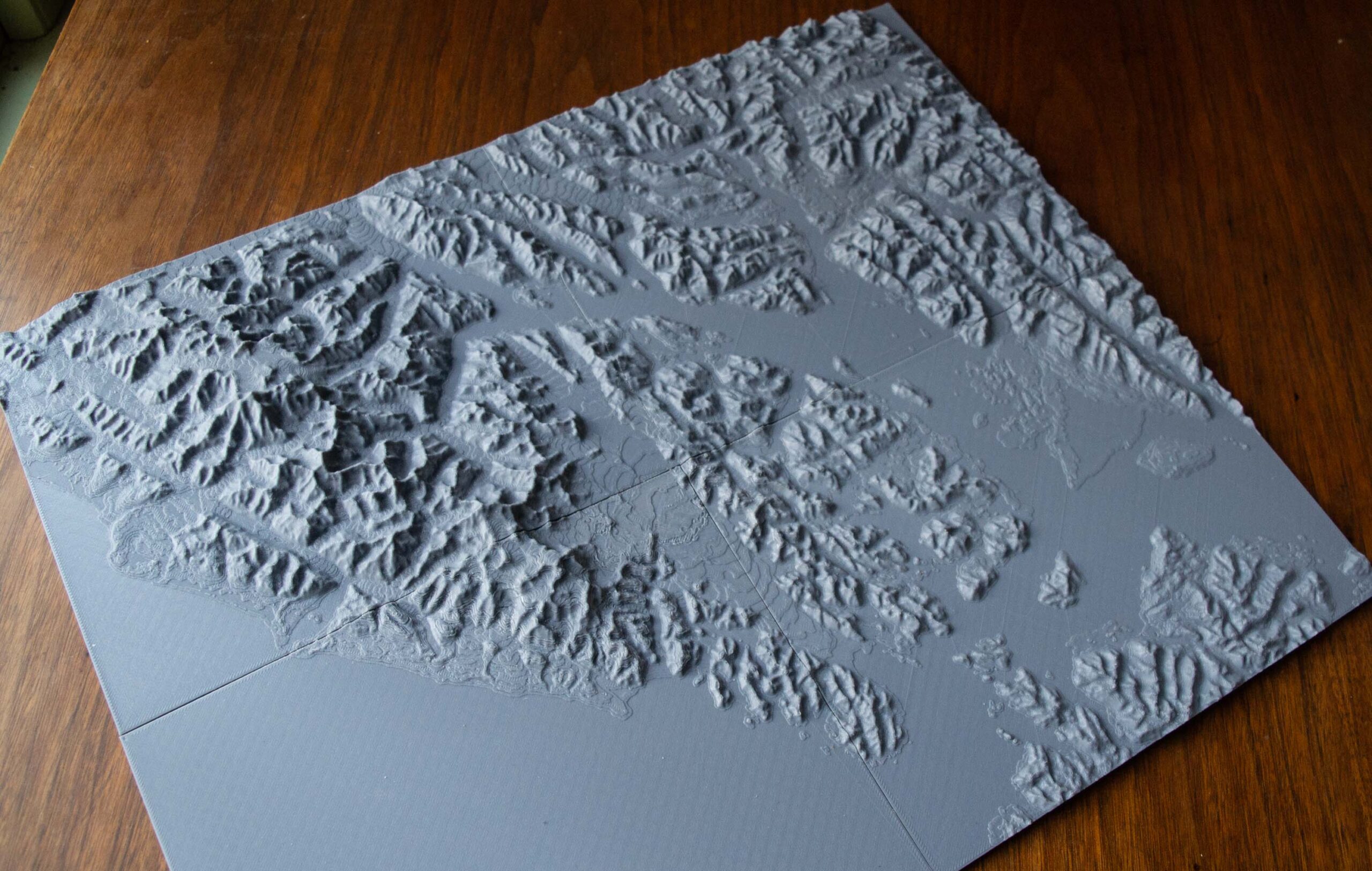
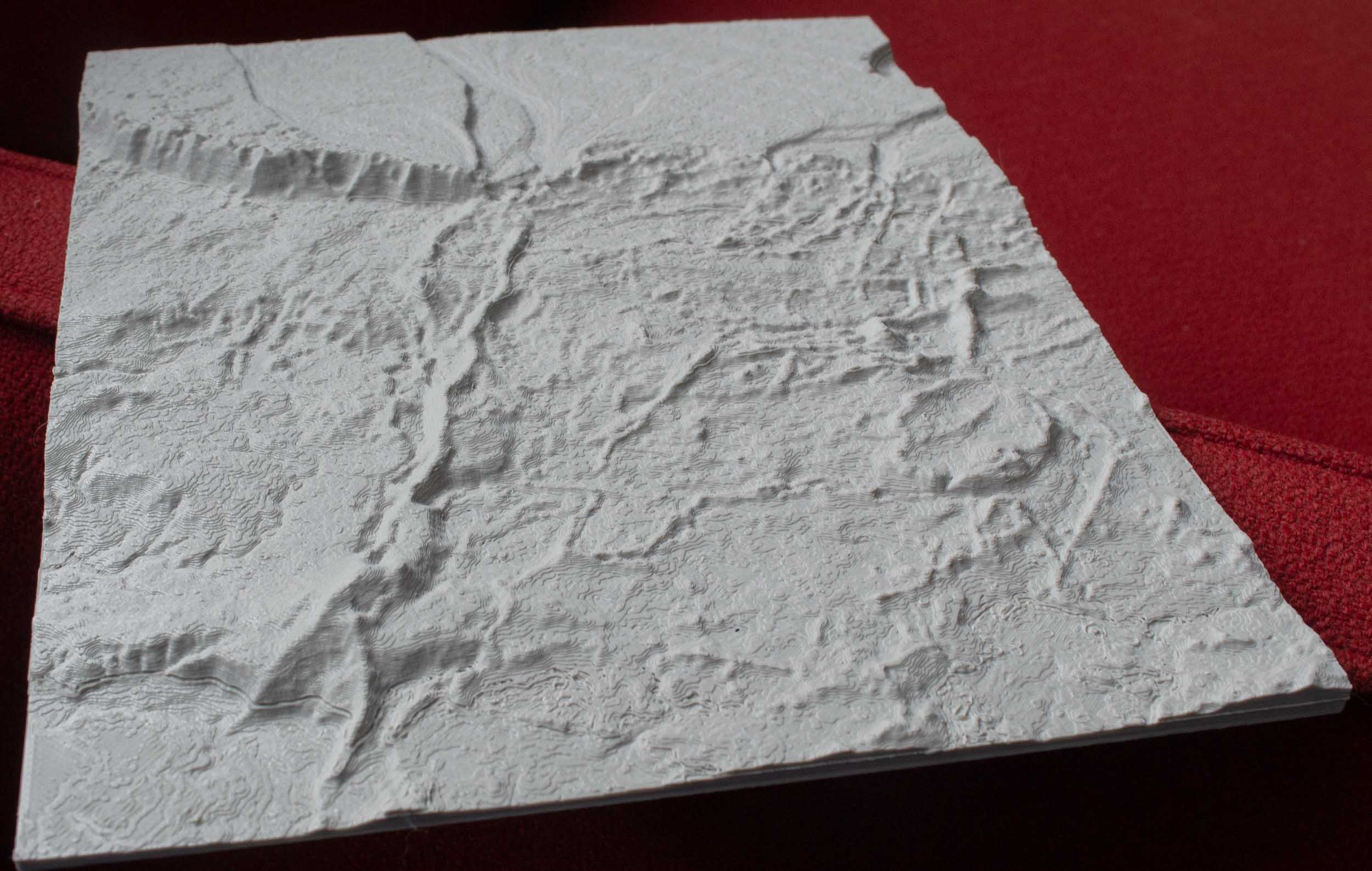
With high resolution LiDAR data, a bigger printer can make intriguing objects. Vermont acquired good LiDAR for the entire state which is now at opentopography.org where one can select a map area (which can include parts of multiple tiles) and download various data types (e.g., bare-earth or first returns) in a few different formats (e.g., point cloud [LAS] or raster surfaces [TIN]). There are options to remove noise from the data and make other tweaks as your order is prepared. I got carried away printing areas of complex 13,000 year-old glacial geomorphology near my house.
Converting the LiDAR raster file from opentopography.org to a file that a 3D printer can use requires a couple of steps. There is a plugin for QGIS (DEMto3D) which produces an stl file from a raster layer. Every 3D printer has a “slicer” program associated with it that converts the stl file to the gcode instructions for the printer.
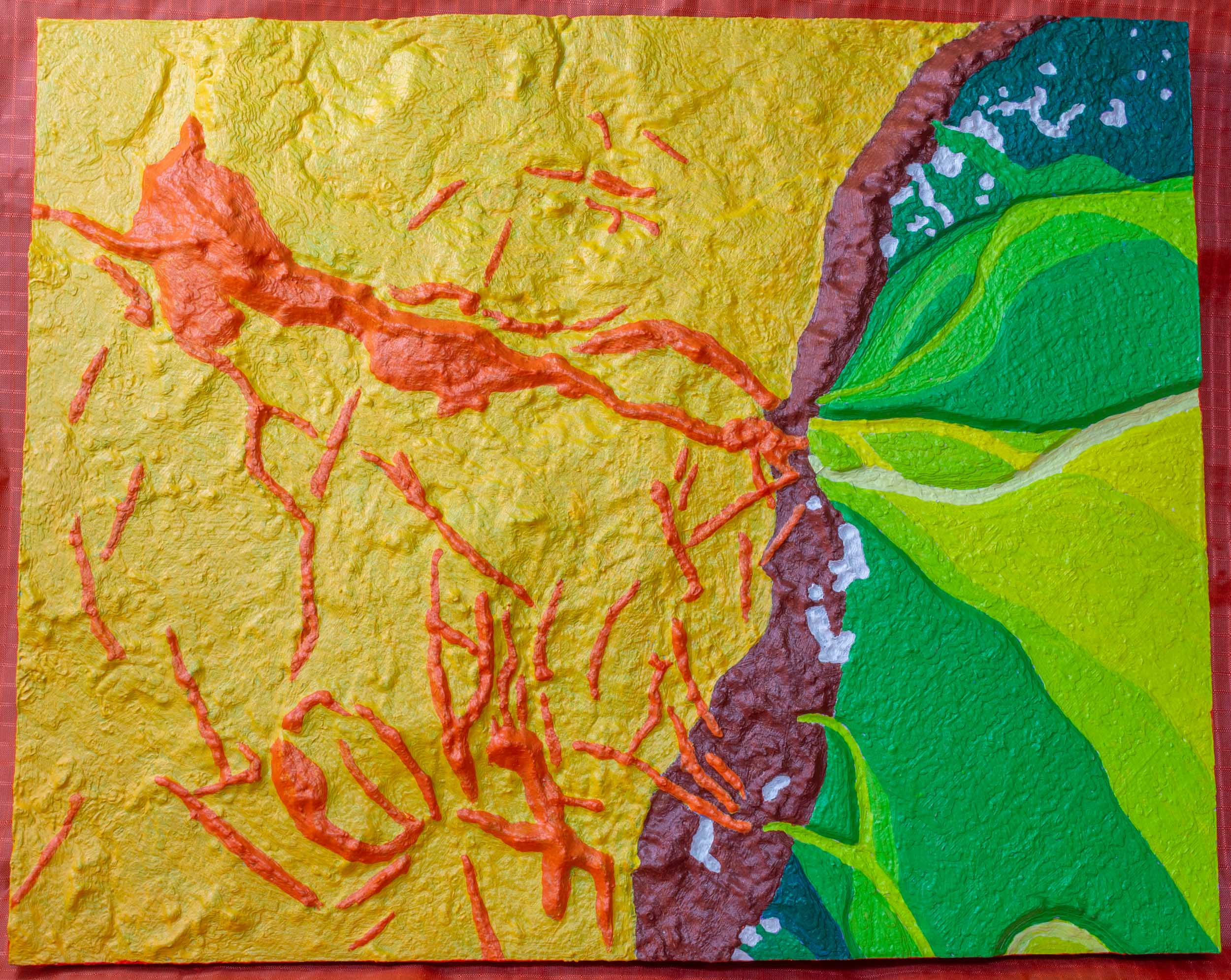
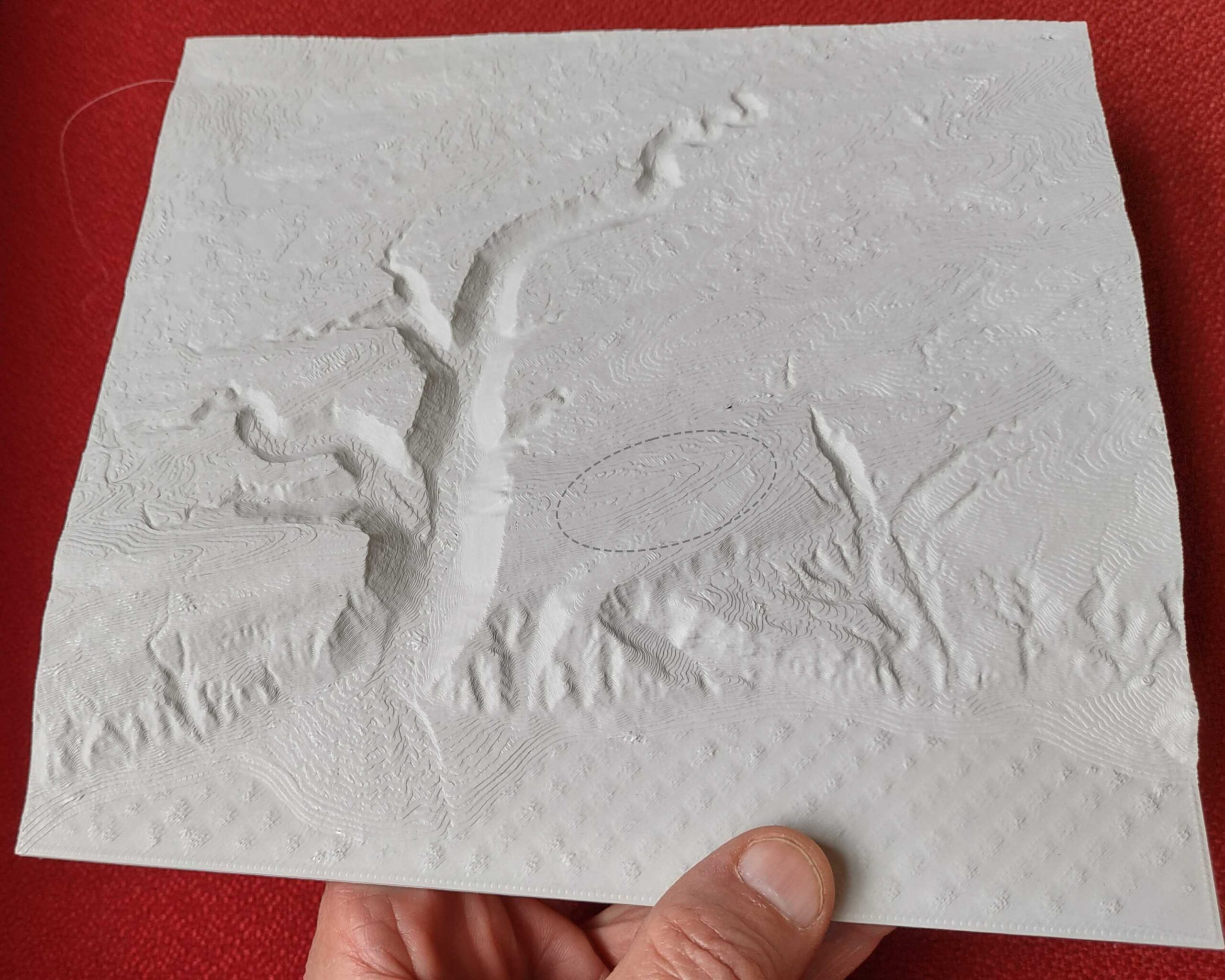
The geomorphological interpretation represented in Figure 8 is somewhat hypothetical. I did not know those orange surfaces were not ca. 1750 outwash until I saw the new LiDAR data and heard from Streveler that there was some reason to believe that they are deformed remnants of a much older outwash surface that was deposited long before the ice reached the terminal moraine. Some of the orange terrain in Figure 8 is higher than the ca. 1750 terminal moraine which is not consistent with it being outwash deposited ca. 1750. I like the Glacio-tectonic Beardslee Formation Deformation Hypothesis and am sticking with it. I want to print a wider view showing all of the putative Beardslee Formation distal to the moraine, but those LiDAR data are not yet at opentopography.org and the USGS National Map site has been down for a week.
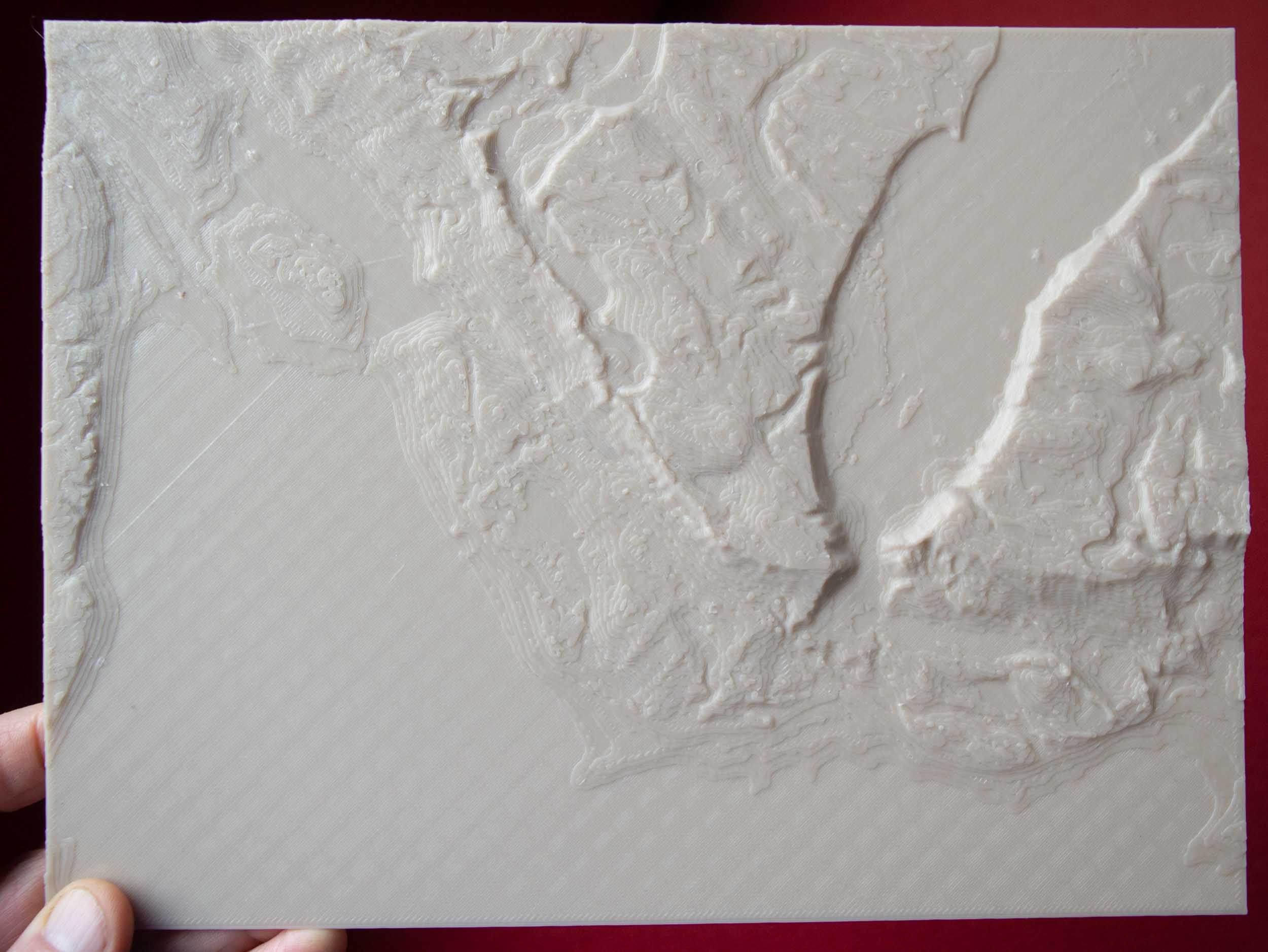
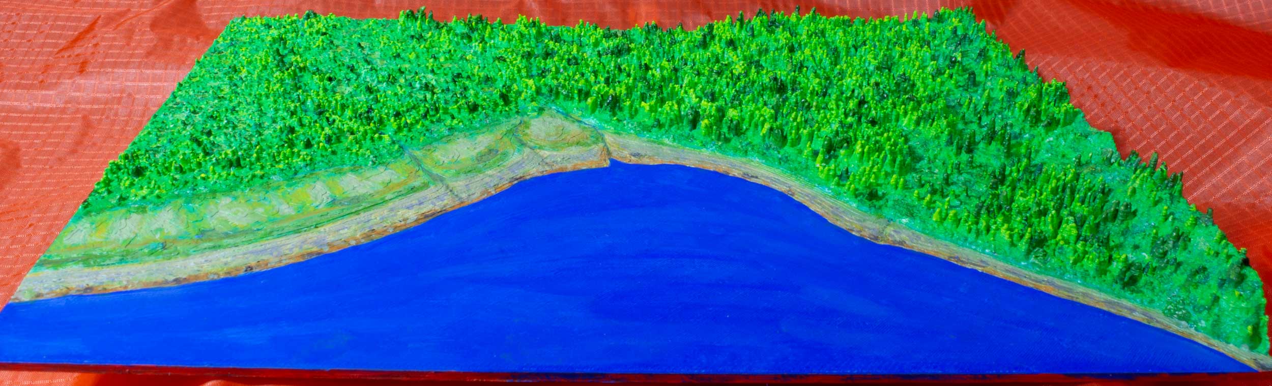
It is also possible to 3D print relief maps with the LiDAR first returns included. The surface of such maps would be covered with a model of the vegetation growing at the site. One of the products available from opentopography.org is a raster layer (TIN) with the first returns point cloud converted to a continuous surface. I don’t know how to convert a point cloud into a continuous surface, so thank you opentopography.org.

Printing a plastic forest is tricky for a couple of reasons. The printer nozzle must skip from tree to tree extruding molten plastic for each tree but none in-between trees. This requires a perfect setting for ooze control that I have not yet found for the new printer (Figure 10). Also, the common 3D printers build up from the bottom by applying plastic in layers and have only limited capability to print shapes that quickly get wider from bottom to top. So spruce trees are easy to print but cottonwood trees, or any lollipop shape are harder. The QGIS plugin that makes the stl file might be solving this problem by making all trees look like Christmas trees. One way or another, all the LiDAR-based 3D printed forests I have made look like spruce forests even when they are maple or oak forests.

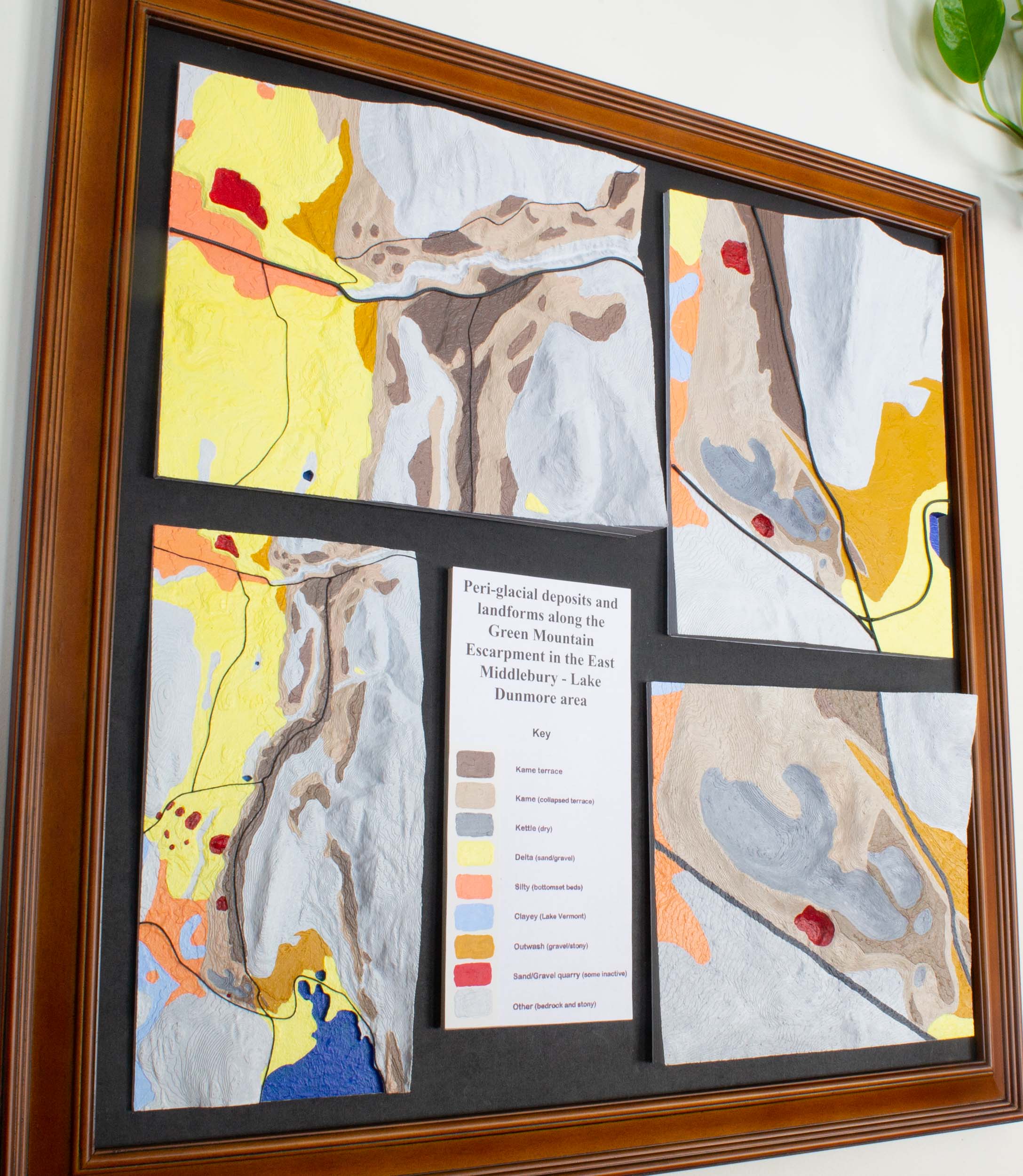
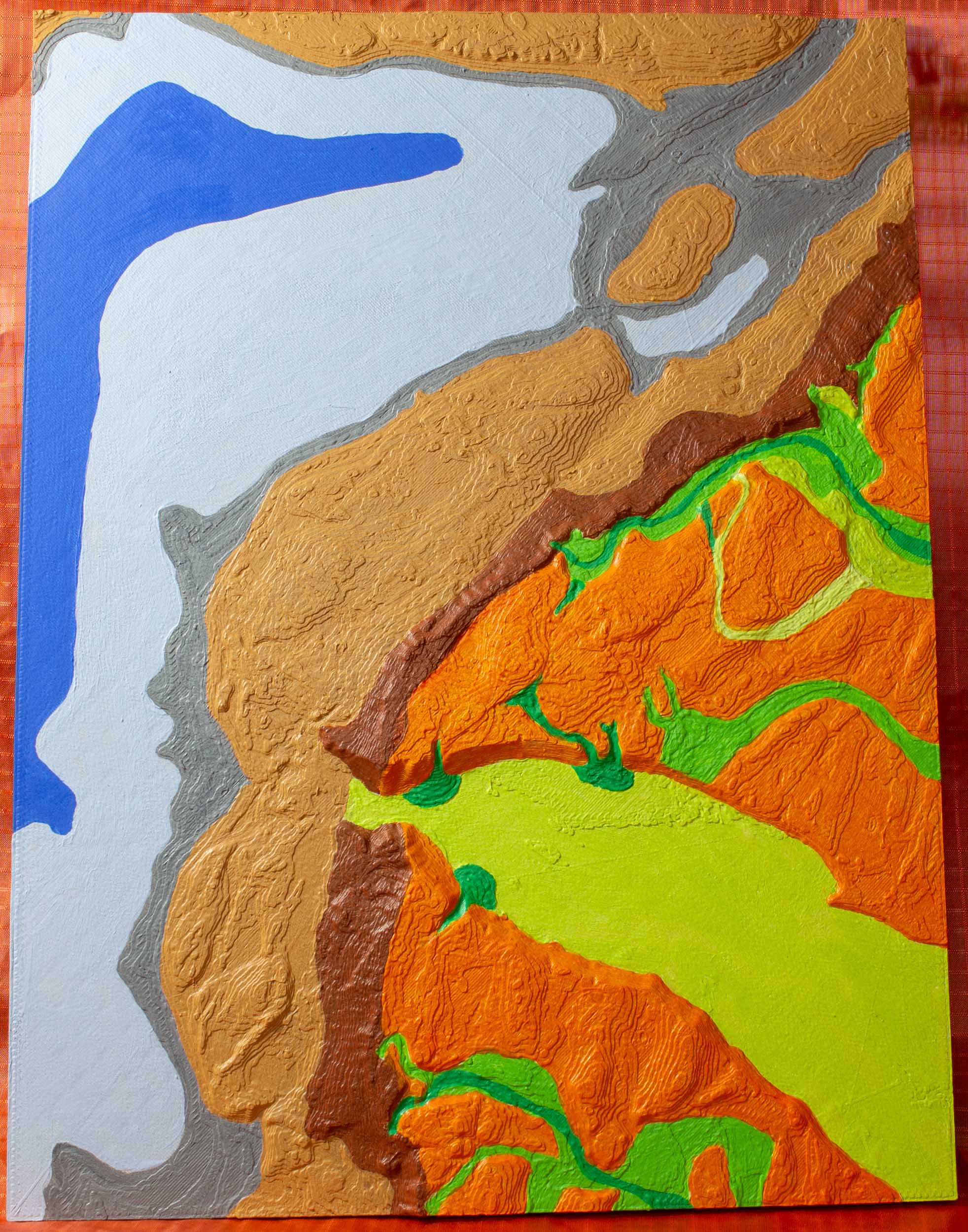
The 10 inch panels have great potential as teaching tools in the field to show the geographic context of natural features. They might be most important for geology and geomorphology students where forests obscure the greater landscape view. Hand-painting the panels is a big task but could also be part of the educational process. Acrylic paints are cheap and easy to use and you can quickly paint draft versions and then paint over your mistakes until you get it right (most of the panels above have at least three different colored coats of paint). When you do get it right there is also the potential for displaying the panels as curiosities or artwork (for the more talented among us).
It takes from five to 15 hours apiece to print these panels. But to a 3D printer, time and plastic are cheap, and I have a pile of prints waiting to be painted. Let me know if you would like to help — the panels are easy to mail. Do you have a favorite place in Glacier Bay you would like to have sitting on your desk?
What do you paint them with? I’d love to have some panels to paint.
I have been using acrylic artists’ paint. It seems to stick well and it’s fun to use.
For some reason I have unpainted prints of the Fred site (Figure 1 above), Site 1 (Figure 1 here: http://fastie.net/lidar-canopies/), and Morse Creek (Figure 3 here: http://fastie.net/bare-earth/). I also have prints of Bartlett Cove (Cooper’s Notch) that I started to paint and then abandoned (Figure 8 above and also farther west). It’s easy to paint over my first failed sketchings.
The four panels in Figure 3 (above) are in Gustavus because I sent them to Ellie (with paints!) but I’m sure she never got a brush wet (to busy with those quilts). So you could negotiate for them.
Let me know and I’ll send them all to you.
Uh… wow. These are beautiful.